Page 197 - Electromagnetics

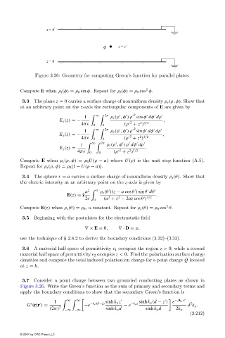
Figure 3.26: Geometry for computing Green’s function for parallel plates.

2
Compute E when ρ l (φ) = ρ 0 sin φ. Repeat for ρ l (φ) = ρ 0 cos φ.
3.3 The plane z = 0 carries a surface charge of nonuniform density ρ s (ρ, φ). Show that
at an arbitrary point on the z-axis the rectangular components of E are given by
2

1 ∞ 2π ρ s (ρ ,φ )ρ cos φ dφ dρ

E x (z) =− ,
2
2 3/2
4π 0 0 (ρ + z )
2

1 ∞ 2π ρ s (ρ ,φ )ρ sin φ dφ dρ
E y (z) =− ,
2
4π 0 0 (ρ + z )
2 3/2

z ∞ 2π ρ s (ρ ,φ )ρ dφ dρ

E z (z) = .
2
4π 0 0 (ρ + z )
2 3/2
Compute E when ρ s (ρ, φ) = ρ 0 U(ρ − a) where U(ρ) is the unit step function (A.5).
Repeat for ρ s (ρ, φ) = ρ 0 [1 − U(ρ − a)].
3.4 The sphere r = a carries a surface charge of nonuniform density ρ s (θ). Show that
the electric intensity at an arbitrary point on the z-axis is given by
a 2 π ρ s (θ )(z − a cos θ ) sin θ dθ

E(z) = ˆ z .
3/2
2
2
2 0 (a + z − 2az cos θ )
2
Compute E(z) when ρ s (θ) = ρ 0 , a constant. Repeat for ρ s (θ) = ρ 0 cos θ.
3.5 Beginning with the postulates for the electrostatic field
∇× E = 0, ∇· D = ρ,
use the technique of § 2.8.2 to derive the boundary conditions (3.32)–(3.33).
3.6 A material half space of permittivity 1 occupies the region z > 0, while a second
material half space of permittivity 2 occupies z < 0. Find the polarization surface charge
densities and compute the total induced polarization charge for a point charge Q located
at z = h.
3.7 Consider a point charge between two grounded conducting plates as shown in
Figure 3.26. Write the Green’s function as the sum of primary and secondary terms and
apply the boundary conditions to show that the secondary Green’s function is
1 ∞ ∞ sinh k ρ z sinh k ρ (d − z ) e − jk ρ ·r

s −k ρ (d−z) −k ρ z 2
G (r|r ) = −e − e d k ρ .
(2π) 2 −∞ −∞ sinh k ρ d sinh k ρ d 2k ρ
(3.212)
© 2001 by CRC Press LLC