Page 287 - Elements of Chemical Reaction Engineering 3rd Edition

Sec. 5.5 Least-Squares Analysis
0.95 conf .
Cower qed 1 ouer upper
1-m , Ualue interval limit limit
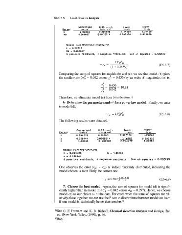
k 2.00878 0.2661 98 1.74259 2.27498
Ke 0.361667 0,0623113 0.293356 0.423979

Plodel: r a=krPexPh?/(i +KerPdA2
k = 2.OC1878
Ke = 0.361667
5 positive residuals, 4 neqative residuals. Sum of squares = 0.436122

(E5 -6.7)

Comparing the sums of squares for models (b) and (c), we see that model (b) gives
2
2
the smaller suim (0, = 0.042 versus ac = 0.436) by an order of magnitude, thlat is,

Therefore, we eliminate model (c) from consideration.I2
6. Determnne the parameters and a2 for a power law model. Finally, we enter
in model (d).

-rA = kPiPk (E5-6.8)
The following results were obtained.

0.95 conf .
Cunver qed louer upper
Par,Z. Ualue 1 nt er Val limit limlt
k 0.894025 0.256901 0.637124 1.15033
a 0.258441 0.070891 4 o. 1 e755 0.329332
b 1.06155 0.209307 0.8522+6 1.27086

Hodel: ra=L:xPeAaxPh2"b
k = 0.894025 b = 1.06155
a = 0.258441
5 posltive residuals, 4 neqarive residuals. Sum of- squares = 0.297'223

One observes the error (rrm - rrc) is indeed randomly distributed, indicating the
model chosen is most likely the correct one.

0.26 1.06
-rA = O.89PE P, (E5-6.9)
7,, Choose the best model. Again, the sum of squares for model (d) is signifi-
cantly higher than in model (b) (a, = 0.042 versus uD = 0.297). Hence, we choose
model (b) as our choice to fit the data. For cases when the sums of squares are rel-
atively close together, we can use the F-test to discriminate between models to learn
if one model is statistically better than another.l3

"See G. F. Froment and K. B. Bishoff, Chemical Reaction Analysis atzd Design, 2nd
ed. (Niew York: Wiley, (1990), p. 96.
131bid! I