Page 283 - Elements of Chemical Reaction Engineering 3rd Edition

Sec. 5.5 Least-Squares Analysis 255

5 I-

k = 5s-'
a=2

I
I
1 2 3 4 5 6 7 8 9 10 11
k
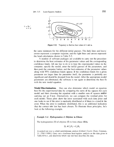
Figure 5-11 Trajectory to find the best values of k and a.

the same minimum for the different initial guesses. The dark lines and heavy
arrows represent a computer trajector, and the light lines and arrows represent
the hand calculations shown in Table 5-2.
A number of software packages are available to carry out the procedure
to determine the best estimates of the parameter values and the corresponding
confidence limits. All one has to do is to type the experimental values in the
computer, specify the model, enter the initial guesses of the parameters, and
then push the computer button, and the best estimates of the parameter values
along with 95% confidence limits appear. If the confidence limits for a given
parameter are larger than the parameter itself, the parameter is probably not
significant and should be dropped from the model. After the appropriate model
parameters are eliminated, the software is run again to determine the best fit
with the new model equation.

Model Discrimination. One can also determine which model or equation
best fits the experimental data by comparing the sums of the squares for each
model and then choosing the equation with a smaller sum of squares andor
carrying out an F-test. Alternatively, we can compare the residual plots for
each model. These plots show the error associated with each data point and
one looks to see if the error is randomly distributed or if there is a trend in( the
error. When the error is randomly distributed, this is an additional indication
that the correct ]rate law has been chosen. To illustrate these principles, let's
look at the following example.

Example 5-6 Hydrogenation of Ethylene to Ethane

The hydrogenation (H) of ethylene (E) to form ethane (EA),

H, + C,H, -+ C,H,
is carried out over a cobalt molybdenum catalyst [CoNecr. Czech. Chem. Commun.,
51, 2760 (198S)l. Carry out a nonlinear least-squares analysis on the data given in
Table E5-6.1, and determine which rate law best describes the data.