Page 281 - Elements of Chemical Reaction Engineering 3rd Edition

Sec. 5.5 Least-Squares Analysis 253

where

s2 = C (r,m - r,Jz
N = number of runs
K = number of parameters to be determined
rrrn = measured reaction rate for run i (i.e., - rAIm)
r,, = calculated reaction rate for run i (i.e~, - rAr,)
To illustrate this technique, let's consider the first-order reaction
A --+ Product

for which we want to learn the reaction order, a, and the specific reaction rate, k,
= kCi

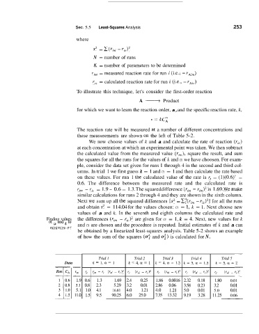
The reaction rate will be measured at a number of different concentrations and
these measurements are shown on the left of Table 5-2.
We now choose values of k and a and calculate the rate of reaction (rlC)
at each concentration at which an experimental point was taken. We then subtract
the calculated value from the measured value ( rllrL), square the result, and sum
the squares for all the runs for the values of k and CY we have choosen. For exam-
ple, consider the data set given for runs 1 through 4 in the second and third col-
umns. In trial 1 we first guess k = 1 and CY = 1 and then calculate the rate based
on these values. For run 1 the calculated value of the rate is r, = (1)(0.6)' =
0.6. The difference between the measured rate and the calculated rate is
Y,, - r,, = 1.9 - 0.6 = 1.3. The squareddifference (rrm - rrm)*is 1.69. Weniake
similar calculations for runs 2 through 4 and they are shown in the sixth column.
Next we sum up all the squared differences [s2 = Cr(r,, - r,,)2] for all the runs
and obtain s2 = 114.04 for the values chosen: CY = 1, k = 1. Next choose new
values of a and k. In the seventh and eighth columns the calculated rate and
Finding values the differences (rflj1 - r,,)2 are given for CY = 1, k = 4. Next, new values for k
Of and to and CY are chosen and the procedure is repeated. Initial estimates of k and a can
rninirmze u2
be obtained by a linearized least-squares analysis. Table 5-2 shows an exarnple
of how the sum of the squares (u: and 0:) is calculated for N.

-
Trial 1 Trial 2 Trial 3 Trial 4 Trial 5
- -
Data k=l,oc=l k=4,a=1 k=4,a=1.5 k=5,cu=1.5 k=5,a=2
r, r, - r, (r, - r,)* r,.
7,
- (r," - r,)* r, (r," - rCl2 r, (r,n - r,)* rc (rm - r,I2
-
-
1.9 0.6 1.3 1.69 2.4 0.25 1.86 0.0016 2.32 0.18 1.80 0.01
3.1 0.8 2.3 5.29 3.2 0.01 2.86 0.06 3.58 0.23 3.2 0.01
5.1 1.0 4.1 16.81 4.0 1.21 4.0 1.21 5.0 0.01 5.0 0.01
11.0 1.5 9.5 90.25 6.0 25.0 7.35 13.32 9.19 3.28 11.25 0.06
--