Page 288 - Elements of Chemical Reaction Engineering 3rd Edition

260 Collection and Analysis of Rate Data Chap. 5

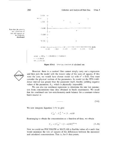
Note that the error is
not ;I functictn of 0
rite ;tnd appearh lo t O
be zindoirily -0.050 1
distributed
-O.l0@ j- 0

-0.15U -+---+--+-----~~ RATE
0.500 1.500 2.500 3.500 4.500 5.500

error = RFiTE - (itPe*PH2,'1"YexPe))
1 = 3.18678
Ke = 2.13133
Figure E5-6.1 F.iior as d lunct~on of calculated rate.

However. there is a caution! One cannot simply carry out a regression
and then pick the model with the lowest value of the sums of squares. If this
were the case, we would have chosen model (a) with u2 = 0.03. One must
consider the physical realism of the parameters. In model (a) the 95% confr-
dence interval was greater than the parameter itself, thereby yielding negative
values of the parameter, Kti, which is physically impossible.
We can also use nonlinear regression to determine the rate law parame-
ters from concentration-time data obtained in batch experiments. We recall
that the combined rate law-stoichiometry-mole balance for a constant-volume
batch reactor is

We now integrate Equation (5-6) to give

I
I
C,4,, - C,, LV = (1 - CX) kt
li
Rearranging to obtain the concentration as ii function of time, we obtain
c, = { ck,;"- (1 - CX)kt]''I-a (5-36)

Now we could use POLYMATH or MATLAB to find the values of CY and k that
would minimize the sum of squares of the differences between the measured
and calculated concentrations. That is, for N data points,