Page 195 - Elements of Distribution Theory

P1: JZP
052184472Xc06 CUNY148/Severini May 24, 2005 2:41

6.3 Moving Average Processes 181

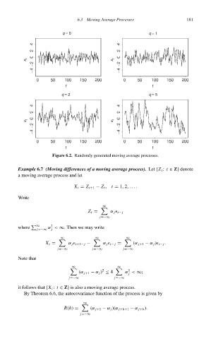
q = 0 q = 1

x t x t
− −
− −

t t
q = 2 q = 5

x t x t
− −
− −

t t
Figure 6.2. Randomly generated moving average processes.

Example 6.7 (Moving differences of a moving average process). Let {Z t : t ∈ Z} denote
amoving average process and let

X t = Z t+1 − Z t , t = 1, 2,....

Write
∞

Z t = α j t− j
j=−∞
2
where ∞ α < ∞. Then we may write
j=−∞ j
∞ ∞ ∞

X t = α j t+1− j − α j t− j = (α j+1 − α j ) t− j .
j=−∞ j=−∞ j=−∞
Note that
∞ ∞
2 2
(α j+1 − α j ) ≤ 4 α < ∞;
j
j=−∞ j=−∞
it follows that {X t : t ∈ Z} is also a moving average process.
By Theorem 6.6, the autocovariance function of the process is given by

∞

R(h) = (α j+1 − α j )(α j+h+1 − α j+h ).
j=−∞