Page 200 - Elements of Distribution Theory

P1: JZP
052184472Xc06 CUNY148/Severini May 24, 2005 2:41

186 Stochastic Processes

Hence, the matrix P (m) with elements P (m) ,i = 1,..., J, j = 1,..., J, satisfies
ij
P (m) = P (r) P (m−r) , r = 0,..., m

m
so that P (m) = P = P ×· · · × P.
Proof. Since the process is assumed to have stationary transition probabilities,

J
(m)
P = Pr(X m = j|X 0 = i) = Pr(X m = j, X r = k|X 0 = i)
ij
k=1
J

= Pr(X m = j|X r = k, X 0 = i)Pr(X r = k|X 0 = i)
k=1
J

= Pr(X m = j|X r = k)Pr(X r = k|X 0 = i)
k=1
J
(m−r) (r)
= P kj P ,
ik
k=1
proving the result.
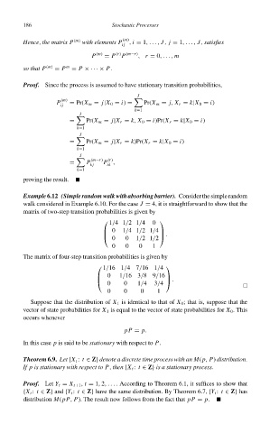
Example 6.12 (Simple random walk with absorbing barrier). Consider the simple random
walk considered in Example 6.10. For the case J = 4, it is straightforward to show that the
matrix of two-step transition probabilities is given by

1/41/21/4 0
 
 0 1/41/21/4 
0 0 1/21/2
  .
0 0 0 1
The matrix of four-step transition probabilities is given by

1/16 1/47/16 1/4
 
 0 1/16 3/89/16 
0 0 1/4 3/4
  .
0 0 0 1
Suppose that the distribution of X 1 is identical to that of X 0 ; that is, suppose that the
vector of state probabilities for X 1 is equal to the vector of state probabilities for X 0 . This
occurs whenever
pP = p.

In this case p is said to be stationary with respect to P.

Theorem 6.9. Let {X t : t ∈ Z} denote a discrete time process with an M(p, P) distribution.
If p is stationary with respect to P, then {X t : t ∈ Z} is a stationary process.

Proof. Let Y t = X t+1 , t = 1, 2,.... According to Theorem 6.1, it suffices to show that
{X t : t ∈ Z} and {Y t : t ∈ Z} have the same distribution. By Theorem 6.7, {Y t : t ∈ Z} has
distribution M(pP, P). The result now follows from the fact that pP = p.