Page 202 - Elements of Distribution Theory

P1: JZP
052184472Xc06 CUNY148/Severini May 24, 2005 2:41

188 Stochastic Processes

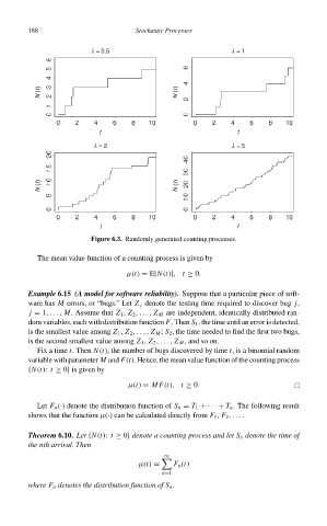
λ = 0.5 λ = 1

N (t) N (t)

t t
λ = 2 λ = 5

N (t) N (t)

t t
Figure 6.3. Randomly generated counting processes.

The mean value function of a counting process is given by
µ(t) = E[N(t)], t ≥ 0.

Example 6.15 (A model for software reliability). Suppose that a particular piece of soft-
ware has M errors, or “bugs.” Let Z j denote the testing time required to discover bug j,
j = 1,..., M. Assume that Z 1 , Z 2 ,..., Z M are independent, identically distributed ran-
dom variables, each with distribution function F. Then S 1 , the time until an error is detected,
is the smallest value among Z 1 , Z 2 ,..., Z M ; S 2 , the time needed to find the first two bugs,
is the second smallest value among Z 1 , Z 2 ,..., Z M , and so on.
Fix a time t. Then N(t), the number of bugs discovered by time t,isa binomial random
variable with parameter M and F(t). Hence, the mean value function of the counting process
{N(t): t ≥ 0} is given by

µ(t) = MF(t), t ≥ 0.

Let F n (·) denote the distribution function of S n = T 1 +· · · + T n . The following result
shows that the function µ(·) can be calculated directly from F 1 , F 2 ,....

Theorem 6.10. Let {N(t): t ≥ 0} denote a counting process and let S n denote the time of
the nth arrival. Then

∞

µ(t) = F n (t)
n=1
where F n denotes the distribution function of S n .