Page 29 - Elements of Distribution Theory

P1: JZP
052184472Xc01 CUNY148/Severini May 24, 2005 17:52

1.5 Quantile Functions 15

It is clear that the approach used in Example 1.14 can be extended to a random variable
of arbitrary dimension. However, the statement of such a result becomes quite complicated.

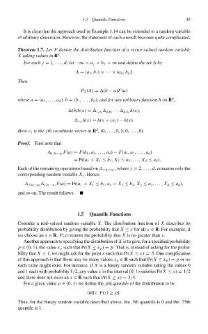
Theorem 1.7. Let F denote the distribution function of a vector-valued random variable
d
X taking values in R .
For each j = 1,..., d, let −∞ < a j < b j < ∞ and define the set A by

A = (a 1 , b 1 ] × ··· × (a d , b d ].
Then

P X (A) = (b − a)F(a)
d
where a = (a 1 ,..., a d ),b = (b 1 ,..., b d ), and for any arbitrary function h on R ,
h(x),
(b)h(x) = 1,b 1 2,b 2 ··· d,b d
j,c h(x) = h(x + ce j ) − h(x).

d
Here e j is the jth coordinate vector in R , (0,..., 0, 1, 0,..., 0).
Proof. First note that

F(a) = F(b 1 , a 2 ,..., a d ) − F(a 1 , a 2 ,..., a d )
1,b 1 −a 1
= Pr(a 1 < X 1 ≤ b 1 , X 2 ≤ a 2 ,..., X d ≤ a d ).
, where j = 2,..., d, concerns only the
Each of the remaining operations based on j,b j −a j
corresponding random variable X j . Hence,
F(a) = Pr(a 1 < X 1 ≤ b 1 , a 2 < X 2 ≤ b 2 , X 3 ≤ a 3 ,..., X d ≤ a d ),
2,b 2 −a 2 1,b 1 −a 1
and so on. The result follows.

1.5 Quantile Functions
Consider a real-valued random variable X. The distribution function of X describes its
probability distribution by giving the probability that X ≤ x for all x ∈ R.For example, if
we choose an x ∈ R, F(x) returns the probability that X is no greater than x.
Another approach to specifying the distribution of X is to give, for a specified probability
p ∈ (0, 1), the value x p such that Pr(X ≤ x p ) = p. That is, instead of asking for the proba-
bility that X ≤ 1, we might ask for the point x such that Pr(X ≤ x) = .5. One complication
of this approach is that there may be many values x p ∈ R such that Pr(X ≤ x p ) = p or no
such value might exist. For instance, if X is a binary random variable taking the values 0
and 1 each with probability 1/2, any value x in the interval [0, 1) satisfies Pr(X ≤ x) = 1/2
and there does not exist an x ∈ R such that Pr(X ≤ x) = 3/4.
Foragiven value p ∈ (0, 1) we define the pth quantile of the distribution to be
inf{z: F(z) ≥ p}.
Thus, for the binary random variable described above, the .5th quantile is 0 and the .75th
quantile is 1.