Page 31 - Elements of Distribution Theory

P1: JZP
052184472Xc01 CUNY148/Severini May 24, 2005 17:52

1.5 Quantile Functions 17

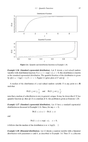
Distribution Function

Q (x)

x
Quantile Function

Q (t)

t
Figure 1.4. Quantile and distribution functions in Example 1.16.

Example 1.16 (Standard exponential distribution). Let X denote a real-valued random
variable with distribution function F(x) = 1 − exp(−x), x > 0; this distribution is known
as the standard exponential distribution. The quantile function of the distribution is given
by Q(t) =− log(1 − t), 0 < t < 1. Figure 1.4 gives plots of F and Q.

A median of the distribution of a real-valued random variable X is any point m ∈ R
such that
1 1
Pr(X ≤ m) ≥ and Pr(X ≥ m) ≥ ;
2 2
note that a median of a distribution is not, in general, unique. It may be shown that if X has
quantile function Q, then Q(.5) is a median of X; this problem is given as Exercise 1.20.

Example 1.17 (Standard exponential distribution). Let X have a standard exponential
distribution as discussed in Example 1.16. Since, for any x > 0,

Pr(X ≤ x) = 1 − Pr(X ≥ x)

and

Pr(X ≥ x) = exp(−x), x > 0,
it follows that the median of the distribution is m = log(2).

Example 1.18 (Binomial distribution). Let X denote a random variable with a binomial
distribution with parameters n and θ,as described in Example 1.4. Then X is a discrete