Page 33 - Elements of Distribution Theory

P1: JZP
052184472Xc01 CUNY148/Severini May 24, 2005 17:52

1.5 Quantile Functions 19

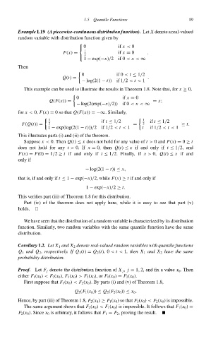
Example 1.19 (A piecewise-continuous distribution function). Let X denote a real-valued
random variable with distribution function given by

 0 if x < 0
1
F(x) = if x = 0 .
2

1 − exp(−x)/2if 0 < x < ∞
Then

0 if 0 < t ≤ 1/2
Q(t) = .
− log(2(1 − t)) if 1/2 < t < 1
This example can be used to illustrate the results in Theorem 1.8. Note that, for x ≥ 0,

0 if x = 0
Q(F(x)) = = x;
− log(2(exp(−x)/2)) if 0 < x < ∞
for x < 0, F(x) = 0so that Q(F(x)) =−∞. Similarly,
1 1

2 if t ≤ 1/2 2 if t ≤ 1/2
F(Q(t)) = = ≥ t.
1 − exp(log(2(1 − t)))/2if 1/2 < t < 1 t if 1/2 < t < 1
This illustrates parts (i) and (ii) of the theorem.
Suppose x < 0. Then Q(t) ≤ x does not hold for any value of t > 0 and F(x) = 0 ≥ t
does not hold for any t > 0. If x = 0, then Q(t) ≤ x if and only if t ≤ 1/2, and
F(x) = F(0) = 1/2 ≥ t if and only if t ≤ 1/2. Finally, if x > 0, Q(t) ≤ x if and
only if
− log(2(1 − t)) ≤ x,

that is, if and only if t ≤ 1 − exp(−x)/2, while F(x) ≥ t if and only if
1 − exp(−x)/2 ≥ t.
This verifies part (iii) of Theorem 1.8 for this distribution.
Part (iv) of the theorem does not apply here, while it is easy to see that part (v)
holds.

We have seen that the distribution of a random variable is characterized by its distribution
function. Similarly, two random variables with the same quantile function have the same
distribution.

Corollary 1.2. Let X 1 and X 2 denote real-valued random variables with quantile functions
Q 1 and Q 2 ,respectively. If Q 1 (t) = Q 2 (t), 0 < t < 1, then X 1 and X 2 have the same
probability distribution.

Proof. Let F j denote the distribution function of X j , j = 1, 2, and fix a value x 0 . Then
either F 1 (x 0 ) < F 2 (x 0 ), F 1 (x 0 ) > F 2 (x 0 ), or F 1 (x 0 ) = F 2 (x 0 ).
First suppose that F 1 (x 0 ) < F 2 (x 0 ). By parts (i) and (v) of Theorem 1.8,
Q 2 (F 1 (x 0 )) ≤ Q 2 (F 2 (x 0 )) ≤ x 0 .

Hence, by part (iii) of Theorem 1.8, F 2 (x 0 ) ≥ F 1 (x 0 )so that F 1 (x 0 ) < F 2 (x 0 )is impossible.
The same argument shows that F 2 (x 0 ) < F 1 (x 0 )is impossible. It follows that F 1 (x 0 ) =
F 2 (x 0 ). Since x 0 is arbitrary, it follows that F 1 = F 2 , proving the result.