Page 35 - Elements of Distribution Theory

P1: JZP
052184472Xc01 CUNY148/Severini May 24, 2005 17:52

1.6 Density and Frequency Functions 21

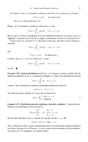
(iii) Suppose that F is absolutely continuous and there exists a function p such that

F (x) = p(x) for almost all x.
Then p is a density function of F.

Proof. If F is absolutely continuous with density p, then
x
F(x) = p(t) dt, −∞ < x < ∞.
−∞
Hence, part (i) follows immediately from the fundamental theorem of calculus, given in
Appendix 1 (Section A1.6). Part (ii) is simply a restatement of result (2) of Section A1.6.
To prove part (iii), note that if F is absolutely continuous, then there exists a function f
such that
x

F(x) = f (t) dt, −∞ < x < ∞
−∞
and

F (x) = f (x) for almost all x.
It follows that f (x) = p(x) for almost all x so that
x
F(x) = p(t) dt, −∞ < x < ∞,
−∞
as well.

Example 1.20 (Uniform distribution on (0, 1)). Let X denote a random variable with the
uniform distribution on (0, 1), as defined in Example 1.9. Then X has distribution function
x
F(x) = dt, 0 ≤ x ≤ 1
0
so that X has an absolutely continuous distribution with density function

p(x) = 1, 0 ≤ x ≤ 1.
Note that the density function of X may also be taken to be
1if 0 < x < 1

p(x) = .
0 otherwise
Example 1.21 (Distribution function satisfying a Lipschitz condition). Consider the dis-
tribution with distribution function given by
0 if x < 1

F(x) = (x − 1) 2 if 1 ≤ x ≤ 2 .
1 if x > 2
We first show that there exists a constant M such that, for all x 1 , x 2 ∈ R,
|F(x 2 ) − F(x 1 )|≤ M|x 2 − x 1 |.

This is called a Lipschitz condition and it implies that F is an absolutely continuous function
and, hence, that part (iii) of Theorem 1.9 can be used to find the density of the distribution;
see Section A1.5 of Appendix 1 for further details.