Page 37 - Elements of Distribution Theory

P1: JZP
052184472Xc01 CUNY148/Severini May 24, 2005 17:52

1.6 Density and Frequency Functions 23

Hence, p(x) can be viewed as being proportional to the probability that X lies in a small
interval containing x;of course, such an interpretation only gives an intuitive meaning to
the density function and cannot be used in formal arguments. It follows that the density
function gives an indication of the relative likelihood of different possible values of X.For
instance, Figure 1.5 shows that the likelihood of X taking a value x in the interval (1, 2)
increases as x increases.
Thus, when working with absolutely continuous distributions, density functions are
often more informative than distribution functions for assessing the basic properties of
a probability distribution. Of course, mathematically speaking, this statement is nonsense
since the distribution function completely characterizes a probability distribution. However,
for understanding the basic properties of the distribution of random variable, the density
function is often more useful than the distribution function.

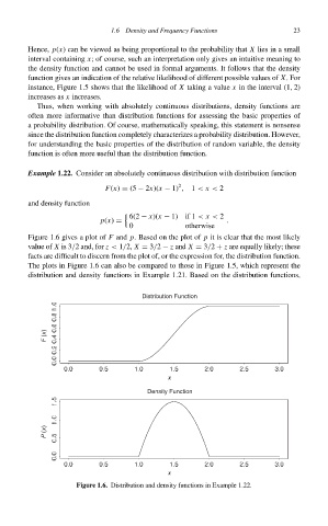
Example 1.22. Consider an absolutely continuous distribution with distribution function
2
F(x) = (5 − 2x)(x − 1) , 1 < x < 2
and density function
6(2 − x)(x − 1) if 1 < x < 2

p(x) = .
0 otherwise
Figure 1.6 gives a plot of F and p. Based on the plot of p it is clear that the most likely
value of X is 3/2 and, for z < 1/2, X = 3/2 − z and X = 3/2 + z are equally likely; these
facts are difficult to discern from the plot of, or the expression for, the distribution function.
The plots in Figure 1.6 can also be compared to those in Figure 1.5, which represent the
distribution and density functions in Example 1.21. Based on the distribution functions,

Distribution Function

F (x)

x

Density Function

P (x)

x
Figure 1.6. Distribution and density functions in Example 1.22.