Page 36 - Elements of Distribution Theory

P1: JZP
052184472Xc01 CUNY148/Severini May 24, 2005 17:52

22 Properties of Probability Distributions

Distribution Function

F (x)

x
Density Function

P (x)

x
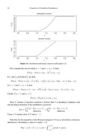
Figure 1.5. Distribution and density functions in Example 1.21.
First consider the case in which x 1 < 1 and 1 ≤ x 2 ≤ 2; then

2
|F(x 2 ) − F(x 1 )|= (x 2 − 1) ≤|x 2 − x 1 |.
If x 1 and x 2 are both in [1, 2], then
2
2
|F(x 2 ) − F(x 1 )|= x − x + 2(x 1 − x 2 ) ≤|x 1 + x 2 + 2||x 2 − x 1 |≤ 6|x 2 − x 1 |;

2 1
if x 2 > 1 and 1 < x 2 < 2, then

2
|F(x 2 ) − F(x 1 )|= 1 − (x 2 − 1) 2 = x − 2x 2 = x 2 |x 2 − 2|≤ 2|x 2 − x 1 |.

2
Finally, if x 1 < 1 and x 2 > 2,
|F(x 2 ) − F(x 1 )|≤ 1 ≤|x 2 − x 1 |.
Since F satisfies a Lipschitz condition, it follows that F is absolutely continuous and
that the density function of the distribution is given by
F (x)if 1 < x < 2 2(x − 1) if 1 < x < 2

p(x) = = .
0 otherwise 0 otherwise
Figure 1.5 contains plots of F and p.

Note that, by the properties of the Riemann integral, if X has an absolutely continuous
distribution with density p, then, for small > 0,
x+ /2 .
Pr(x − /2 < X < x + /2) = p(t) dt = p(x) .
x− /2