Page 30 - Elements of Distribution Theory

P1: JZP
052184472Xc01 CUNY148/Severini May 24, 2005 17:52

16 Properties of Probability Distributions

The quantile function of the distribution or, more simply, of X,is the function Q :
(0, 1) → R given by
Q(t) = inf{z: F(z) ≥ t}.

The quantile function is essentially the inverse of the distribution function F;however,
since F is not necessarily a one-to-one function, its inverse may not exist. The pth quantile
of the distribution, as defined above, is given by Q(p), 0 < p < 1.

Example 1.15 (Integer random variable). Let X denote a random variable with range
X ={1, 2,..., m} for some m = 1, 2,..., and let

θ j = Pr(X = j), j = 1,..., m.

The distribution function of X is given in Example 1.11; it is a step function with jump θ j
at x = j.
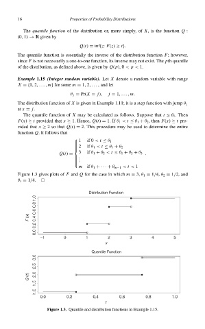
The quantile function of X may be calculated as follows. Suppose that t ≤ θ 1 . Then
F(x) ≥ t provided that x ≥ 1. Hence, Q(t) = 1. If θ 1 < t ≤ θ 1 + θ 2 , then F(x) ≥ t pro-
vided that x ≥ 2so that Q(t) = 2. This procedure may be used to determine the entire
function Q.It follows that
1 if 0 < t ≤ θ 1


 2 if θ 1 < t ≤ θ 1 + θ 2



3 if θ 1 + θ 2 < t ≤ θ 1 + θ 2 + θ 3 .
Q(t) =
 .
 .
 .


m if θ 1 +· · · + θ m−1 < t < 1
Figure 1.3 gives plots of F and Q for the case in which m = 3, θ 1 = 1/4, θ 2 = 1/2, and
θ 3 = 1/4.
Distribution Function

F (x)

−
x
Quantile Function

Q (t)

t
Figure 1.3. Quantile and distribution functions in Example 1.15.