Page 570 - Elements of Chemical Reaction Engineering Ebook

540 Unsteady-State Nonisothermal Reactor Design Chap. 9

Hand Calculation
Integrating Equation (E9-1.3) gives

(E9- 1.7)

Again, the variation of Simpson's rule used in Example 8-6 is used. We now
choose X, calculate T from Equation (E9- 1.6), calculate k, and then calculate
(1 / [k( 1 - X)]) and tabulate it in Table E9- 1.1.

TABLE E9- 1.1

-
-~
0 535 2.73 x 10-4 3663 = fo
0.1288 547 5.33 x 10-4 2154 = fi
0.2575 558 9.59 x 10-4 1404 = f2
0.3863 570 17.7 x 10-4 921 = f3
0.5150 582 32.0 x 10-4 644 = f4

In evaluating Equation (E9- 1.7) numerically, it was decided to use four
equal intervals. Consequently, hx = h = 0.515/4 = 0.12875. Using Simp-
son's rule, we have

= (0.12875)[3663 + (4)(2154) + (2)(1404) + (4)(921) + 6441
3
= 833 s or 13.9 rnin

T = 582 R or 122°F

Computer Solution
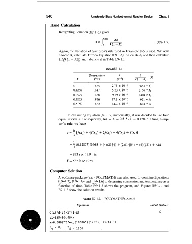
A software package (e.g., POLYMATH) was also used to combine Equations
(E9-1.3), (E9-1.4)> and (E9- 1.6) to determine conversion and temperature as a
function of time. Table E9-1.2 shows the program, and Figures E9-1.1 and
E9-1.2 show the solution results.

TABLE E9-1.2. POLYMATH PROGRAM
Equations: Initial Values:
0