Page 108 - Academic Press Encyclopedia of Physical Science and Technology 3rd Polymer

P1: FMX/LSU P2: GPB/GRD P3: GLQ Final pages
Encyclopedia of Physical Science and Technology EN012c-593 July 26, 2001 15:56

614 Polymer Processing

FIGURE 3 Shear stress versus velocity gradient or shear rate for
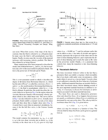
several different types of fluids. [From Baird, D. G., and Collias, D. I. FIGURE 4 Viscosity versus shear rate (i.e., flow curves) for a
(1998). “Polymer Processing: Principles and Design,” Wiley, metallocene catalyzed polyethylene at temperatures of 170 and
◦
New York.] 190 C.

−1
can occur. When flow occurs, if the slope of the line is values (e.g., >10,000 sec ) and for polymer melts this
constant, then the fluid is referred to as a Bingham fluid. can be taken as zero; λ has units of seconds and approx-
In many cases the fluid is still pseudoplastic once flow imately represents the reciprocal of the shear rate for the
begins. Finally, in some cases the viscosity of the material onset of shear thinning behavior; and n represents the de-
increases with increasing velocity gradient. The fluid is gree of shear thinning and is nearly the same as the value
then referred to as being dilatant. in the power-law model. Finally, a is a parameter that
Many empiricisms have been proposed to describe the controls how sharp the transition is into shear-thinning
steady state relation between τ yx and dv x /dy, but we men- behavior.
tion only a few of the most useful for polymeric fluids. The
B. Viscoelastic Behavior
first is the power law of Ostwald and de Waele:
The term viscoelastic behavior refers to the fact that a
n−1
dv x
η = m . (4) polymeric fluid can exhibit a response which resembles
dy that of an elastic solid under some circumstances, while

This is a two-parameter model in which n describes the under others it can act as a viscous liquid. Viscosity alone
degree of deviation from Newtonian behavior; m, which is not sufficient to describe the flow behavior of polymer
n
has the units of Pa sec , is called the consistency.For n = 1 melts. Additional material functions are needed which re-
and m = µ, this model predicts Newtonian fluid behavior. flect their viscoelastic nature. Before defining several of
For n < 1, the fluid is pseudoplastic while for n > 1 the the most important material functions in addition to vis-
fluid is dilatant. It particular, the model describes the vis- cosity, it is necessary to discuss the kinematics or defor-
cosity behavior as shown in Fig. 4 in the region where the mation associated with these material functions.
viscosity decreases linearly with increasing velocity gra- Two basic flows are used to characterize polymers:
dient (which is also called shear rate). The curves shown shear and shear-free flows. (It so happens that processes
in Fig. 4 are also referred to as flow curves. Actually most are usually a combination of these flows or sometimes are
polymeric fluids exhibit a constant viscosity at low shear dominated by one type or the other.) The velocity field for
rates and then shear thin at higher shear rates (Fig. 4). rectilinear shear flow (Fig. 2) is given below:
A model that is used often in numerical calculations, be- v x = ˙γ (t)y v y = v z = 0, (6)
cause it fits the full flow curve, is the Carreau–Yasuda
model: where ˙γ (t) may be constant or a function of time. The
velocity field for shear-free flows can be given in a general
n−1
a
η − η ∞ dv x a form as
= 1 + λ . (5)
dy
v x =−1/2 ˙ε (1 + b)x,
η 0 − η ∞
This model contains five parameters: η 0 , η ∞ , λ, a, and
v y =−1/2 ˙ε (1 − b)y, (7)
n. η 0 is the zero shear viscosity just as above; η ∞ is the
viscosity as the shear rate or dv x /dy goes to very high v z =+ ˙εz,