Page 208 - Engineering Digital Design

4.9 FACTORIZATION, RESUBSTITUTION, AND DECOMPOSITION METHODS 179

As a practical example of the application of Shannon's expansion theorem, consider the
function
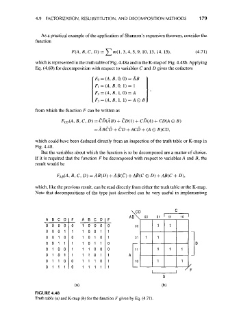
F(A, B, C, D) = ^m(l, 3, 4, 5, 9, 10, 13, 14,15), (4.71)

which is represented in the truth table of Fig. 4.48a and in the K-map of Fig. 4.48b. Applying
Eq. (4.69) for decomposition with respect to variables C and D gives the cofactors
F 0 = (A, B,Q,Q)=AB
F) = (A, 5,0, 1)= 1
F 2 = (A, B, 1,0) = A
F 3 = (A,B,l,l)=AQB\

from which the function F can be written as
F CD(A, B, C, D) = CD(AB) + CD(1) + CD(A) + CD(A Q B)

= ABCD + CD + ACD + (A 0 B)CD,

which could have been deduced directly from an inspection of the truth table or K-map in
Fig. 4.48.
But the variables about which the function is to be decomposed are a matter of choice.
If it is required that the function F be decomposed with respect to variables A and B, the
result would be

F AB(A, B, C, D) = AB(D)+AB(C)+AB(C 0 D) + AB(C + D),

which, like the previous result, can be read directly from either the truth table or the K-map.
Note that decompositions of the type just described can be very useful in implementing

VCD °
00 01 11 10
AB
A B C D F A B C D F \
000 0 0 100 0 0 00 1 1
000 1 1 100 1 1
001 0 0 101 0 1 01 1 1
001 1 1 101 1 0
010 0 1 110 0 0 11 1 1 1
010 1 1 110 1 1 A
011 0 0 111 0 1 10 1 1
011 1 0 111 1 1 /
/ F

(a) (b)
FIGURE 4.48
Truth table (a) and K-map (b) for the function F given by Eq. (4.71).