Page 773 - Engineering Digital Design

14.15 PERSPECTIVE ON STATE CODE ASSIGNMENTS 739

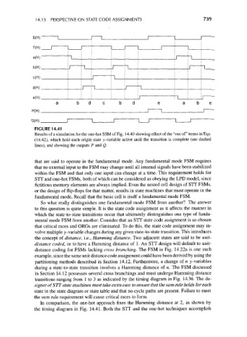
S(H)
T(H)

a(H)
b(H)

c(H).
d(H)

e(H)

P(H)

Q(H).
FIGURE 14.41
Results of a simulation for the one-hot SSM of Fig. 14.40 showing effect of the "out of" terms in Eqs.
(14.42), which hold each origin state ^-variable active until the transition is complete (see dashed
lines), and showing the outputs P and Q.

that are said to operate in the fundamental mode. Any fundamental mode FSM requires
that no external input to the FSM may change until all internal signals have been stabilized
within the FSM and that only one input can change at a time. This requirement holds for
STT and one-hot FSMs, both of which can be considered as obeying the LPD model, since
fictitious memory elements are always implied. Even the nested cell design of STT FSMs,
or the design of flip-flops for that matter, results in state machines that must operate in the
fundamental mode. Recall that the basic cell is itself a fundamental mode FSM.
So what really distinguishes one fundamental mode FSM from another? The answer
to this question is quite simple. It is the state code assignment as it affects the manner in
which the state-to-state transitions occur that ultimately distinguishes one type of funda-
mental mode FSM from another. Consider that an STT state code assignment is so chosen
that critical races and ORGs are eliminated. To do this, the state code assignment may in-
volve multiple y-variable changes during any given state-to-state transition. This introduces
the concept of distance, i.e., Hamming distance. Two adjacent states are said to be unit-
distance coded, or to have a Hamming distance of 1. An STT design will default to unit-
distance coding for FSMs lacking cross branching. The FSM in Fig. 14.22a is one such
example, since the same unit distance code assignment could have been derived by using the
partitioning methods described in Section 14.12. Furthermore, a change of n y-variables
during a state-to-state transition involves a Hamming distance of n. The FSM discussed
in Section 14.12 possesses several cross branchings and must undergo Hamming distance
transitions ranging from 1 to 3 as indicated by the timing diagram in Fig. 14.36. The de-
signer of STT state machines must take extra care to ensure that the sum rule holds for each
state in the state diagram or state table and that no cycle paths are present. Failure to meet
the sum rule requirement will cause critical races to form.
In comparison, the one-hot approach fixes the Hamming distance at 2, as shown by
the timing diagram in Fig. 14.41. Both the STT and the one-hot techniques accomplish