Page 771 - Engineering Digital Design

14.14 ONE-HOT DESIGN OF ASYNCHRONOUS STATE MACHINES 737

coupled terms cST and bcde, indicating (c — > b) under branching conditions ST , but is
covered by the holding condition "into" term bST for state b. The other s-hazard exists in
function Y c and is produced between coupled terms bST and cbe, meaning b — > c under
branching conditions ST, with cover provided by the "into" holding condition term cT for
state c. Thus, hazard cover in the NS logic expression of one-hot designs is provided by
a reduced consensus term, which turns out to be the "into" holding condition term of the
state for which the NS function applies. If left active, s-hazards in the NS logic can cause
malfunction of the FSM. No s-hazard is possible in the Q output function of Eqs. (14.42),
since the coupled terms eS and dST indicate an externally initiated static 1 -hazard that
must occur in a two 1 's state under a holding condition T that is clearly not possible in a
one-hot design.
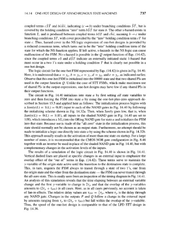
The logic circuit for the one-hot FSM represented by Eqs. (14.42) is given in Fig. 14.40.
Here, it is understood that a = y a , b = y^, c = y c, d = y</, and e = y e, as indicated earlier.
Observe that this one-hot FSM is initialized into the 00000 state and that two shared Pis are
used in the output function Q. Unlike the case of STT FSMs, which make maximum use
of shared Pis in the output expressions, one-hot designs may have few if any shared Pis in
their output functions.
The circuit in Fig. 14.40 initializes into state a by first setting all state variables to
zero and then forcing the FSM into state a by using the one-hot-plus-zero approach de-
scribed in Section 13.5 and applied here as follows: The initialization process begins with
a Sanity(L) = 1(L) = 0(#) input to each of the NAND gates in Fig. 14.40 by following
the initializing scheme shown in Fig. 14.32a. Then, when Sanity goes low, that is, when
Sanity(L) = 0(L) = !(//), all inputs to the shaded NAND gate in Fig. 14.40 are set to
1(H), which introduces a 1(L) into the ORing NAND gate for state a and initializes the FSM
into that state. Because use is made of the "all-zero" state in the initialization process, this
state should normally not be chosen as an output state. Furthermore, no attempt should be
made to initialize a logic one directly into state a by using the scheme shown in Fig. 14.32b.
This approach usually results in the activation of more than one state on startup. For a large
number of states, it is recommended that the CMOS NOR gate configuration in Fig. 8.46
together with an inverter be used in place of the shaded NAND gate in Fig. 14.40, but with
complementary changes in the activation levels of the inputs.
The results of a simulation of the logic circuit in Fig. 14.40 is shown in Fig. 14.41.
Vertical dashed lines are placed at specific changes in an external input to emphasize the
overlap effect of the "out of" terms in Eqs. (14.42). These terms serve to maintain the
y-variable of the origin state active until the transition to the destination state is complete.
This, in turn, requires the FSM always to transit through a state of two 1's, one from
the origin state and the other from the destination state — the FSM can never transit through
the all-zero state. This is easily seen from an inspection of the timing diagram in Fig. 14.41 .
An analysis of this simulation reveals that the time elapsing between an external variable
change and the first y-variable to change is 2r p and that the overlap of the y-variables
amounts to (2r p + t/yvv) in all cases. Here, as in all cases previously, no account is taken
of fan-in effects. The relative delay values are T INV = | T P, where r p is the delay through
any NAND gate. Changes in the outputs P and Q follow a change in the external input
by amounts ranging from T P to (2r p + TINV) but fall within the overlap of the y-variable.
Thus, the speed of the one-hot design is comparable to that of the LPD STT design in
Fig. 14.36.