Page 353 - Engineering Electromagnetics, 8th Edition

CHAPTER 10 Transmission Lines 335

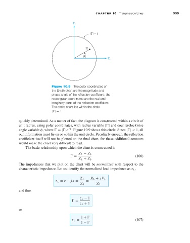
Figure 10.9 The polar coordinates of
the Smith chart are the magnitude and
phase angle of the reflection coefficient; the
rectangular coordinates are the real and
imaginary parts of the reflection coefficient.
The entire chart lies within the circle
| |= 1.

quickly determined. As a matter of fact, the diagram is constructed within a circle of
unit radius, using polar coordinates, with radius variable | | and counterclockwise
angle variable φ, where =| |e . Figure 10.9 shows this circle. Since | | < 1, all
jφ
our information must lie on or within the unit circle. Peculiarly enough, the reflection
coefficient itself will not be plotted on the final chart, for these additional contours
would make the chart very difficult to read.
The basic relationship upon which the chart is constructed is

Z L − Z 0
= (106)
Z L + Z 0
The impedances that we plot on the chart will be normalized with respect to the
characteristic impedance. Let us identify the normalized load impedance as z L ,

Z L R L + jX L
z L = r + jx = =
Z 0 Z 0
and thus
z L − 1
=
z L + 1
or

1 +
z L = (107)
1 −