Page 99 - Essentials of applied mathematics for scientists and engineers

book Mobk070 March 22, 2007 11:7

SOLUTIONS USING FOURIER SERIES AND INTEGRALS 89
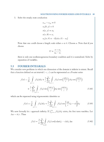
3. Solve the steady-state conduction

u xx + u yy = 0

u x (0, y) = 0

u(a, y) = u 0
u(x, 0) = u 1
u y (x, b) =−h[u(x, b) − u 1 ]

Note that one could choose a length scale either a or b. Choose a. Note that if you
choose

u − u 1
U =
u 0 − u 1
there is only one nonhomogeneous boundary condition and it is normalized. Solve by
separation of variables.

5.3 FOURIER INTEGRALS
We consider now problems in which one dimension of the domain is infinite in extent. Recall
that a function defined on an interval (−c , c ) can be represented as a Fourier series
c c
1 1 nπς nπx
∞
f (x) = f (ς)dς + f (ς)cos dς cos
2c c c c
ς=−c n=1 ς=−c
c
1 nπς nπx
∞
+ f (ς)sin dς sin (5.88)
c c c
n=1 ς=−c
which can be expressed using trigonometric identities as
c c
1 1 nπ
∞
f (x) = f (ς)dς + f (ς)cos (ς − x) dς (5.89)
2c c c
ς=−c n=1 ς=−c
We now formally let c approach infinity. If ∞ f (ς)dς exists, the first term vanishes. Let
ς=−c
α = π/c .Then

c
2
∞
f (x) = f (ς)cos[n α(ς − x)dς α (5.90)
π
n=1
ς=0