Page 199 - Essentials of physical chemistry

More Kinetics and Some Mechanisms 161

GRAPHICAL–ANALYTICAL METHOD FOR DH AND DS z
z
The method above is useful for estimating the Eyring parameters using only two data points in a test
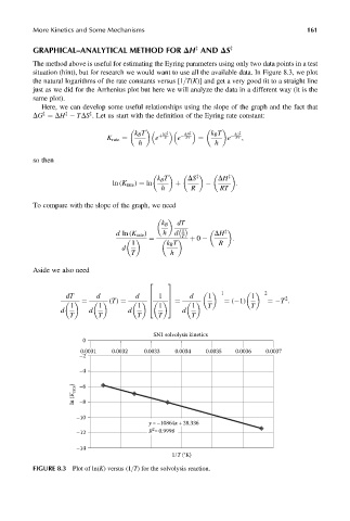
situation (hint), but for research we would want to use all the available data. In Figure 8.3, we plot
the natural logarithms of the rate constants versus [1=T(K)] and get a very good fit to a straight line
just as we did for the Arrhenius plot but here we will analyze the data in a different way (it is the
same plot).
Here, we can develop some useful relationships using the slope of the graph and the fact that
DG ¼ DH TDS . Let us start with the definition of the Eyring rate constant:
z
z
z

k B T DS z DH z k B T DG z
e þ R e RT e RT ,
K rate ¼ ¼
h h
so then

k B T DS z DH z
ln (K rate ) ¼ ln þ :
h R RT
To compare with the slope of the graph, we need

k B dT

1
d ln (K rate ) h d DH z
T
¼ þ 0 :
1 k B T R
d
T h
Aside we also need
2 3
1 2
dT d d 6 1 7 d 1 1 2
¼ (T) ¼ 7 ¼ ¼ ( 1) ¼ T :
6
1 1 1 4 1 5 1 T T
d d d d
T T T T T
SN1 solvolysis kinetics
0
0.0031 0.0032 0.0033 0.0034 0.0035 0.0036 0.0037
–2
–4
ln (K rate ) –6

–8

–10
y =–10864x +28.336
2
R =0.9998
–12
–14
1/T (°K)
FIGURE 8.3 Plot of ln(K) versus (1=T) for the solvolysis reaction.