Page 210 - Essentials of physical chemistry

172 Essentials of Physical Chemistry

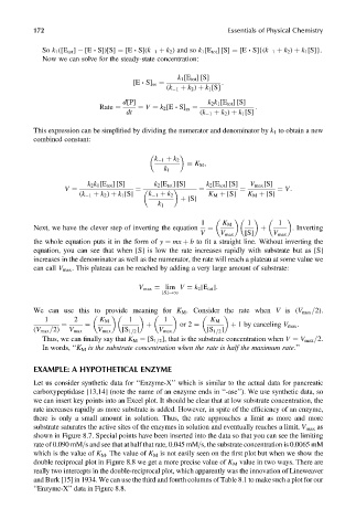
So k 1 ([E tot ] [E S])[S] ¼ [E S](k 1 þ k 2 ) and so k 1 [E tot ] [S] ¼ [E S]{(k 1 þ k 2 ) þ k 1 [S]}.
Now we can solve for the steady-state concentration:

k 1 [E tot ] [S]
:
[E S] ss ¼
(k 1 þ k 2 ) þ k 1 [S]
d[P] k 2 k 1 [E tot ] [S]
:
dt (k 1 þ k 2 ) þ k 1 [S]
Rate ¼ ¼ V ¼ k 2 [E S] ss ¼
This expression can be simplified by dividing the numerator and denominator by k 1 to obtain a new
combined constant:

k 1 þ k 2
K M ,
k 1
k 2 k 1 [E tot ] [S] k 2 [E tot ] [S] k 2 [E tot ] [S] V max [S]
¼ ¼ V:
(k 1 þ k 2 ) þ k 1 [S] k 1 þ k 2 K M þ [S] K M þ [S]
V ¼ ¼ ¼
þ [S]
k 1

1 K M 1 1
Next, we have the clever step of inverting the equation ¼ þ . Inverting
V V max [S] V max
the whole equation puts it in the form of y ¼ mx þ b to fit a straight line. Without inverting the
equation, you can see that when [S] is low the rate increases rapidly with substrate but as [S]
increases in the denominator as well as the numerator, the rate will reach a plateau at some value we
can call V max . This plateau can be reached by adding a very large amount of substrate:

V max ¼ lim V ¼ k 2 [E tot ]:
[S]!1
We can use this to provide meaning for K M . Consider the rate when V is (V max =2).

1 2 K M 1 1 K M
þ 1 by canceling V max .
þ
(V max =2) V max V max [S 1=2 ] V max [S 1=2 ]
¼
¼
or 2 ¼
Thus, we can finally say that K M ¼ [S 1=2 ], that is the substrate concentration when V ¼ V max =2.
In words, ‘‘K M is the substrate concentration when the rate is half the maximum rate.’’
EXAMPLE: A HYPOTHETICAL ENZYME
Let us consider synthetic data for ‘‘Enzyme-X’’ which is similar to the actual data for pancreatic
carboxypeptidase [13,14] (note the name of an enzyme ends in ‘‘-ase’’). We use synthetic data, so
we can insert key points into an Excel plot. It should be clear that at low substrate concentration, the
rate increases rapidly as more substrate is added. However, in spite of the efficiency of an enzyme,
there is only a small amount in solution. Thus, the rate approaches a limit as more and more
substrate saturates the active sites of the enzymes in solution and eventually reaches a limit, V max as
shown in Figure 8.7. Special points have been inserted into the data so that you can see the limiting
rate of 0.090 mM=s and see that at half that rate, 0.045 mM=s, the substrate concentration is 0.0065 mM
which is the value of K M . The value of K M is not easily seen on the first plot but when we show the
double reciprocal plot in Figure 8.8 we get a more precise value of K M value in two ways. There are
really two intercepts in the double-reciprocal plot, which apparently was the innovation of Lineweaver
and Burk [15] in 1934. We can use the third and fourth columns of Table 8.1 to make such a plot for our
‘‘Enzyme-X’’ data in Figure 8.8.