Page 277 - Essentials of physical chemistry

The Schrödinger Wave Equation 239

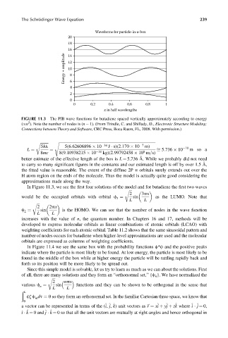
Waveforms for particle-in-a-box
20
18
16
Energy + amplitude 12 8
14

10

4 6
2
0
0 0.2 0.4 0.6 0.8 1
x in half wavelengths
FIGURE 11.3 The PIB wave functions for butadiene spaced vertically approximately according to energy
2
(/n ). Note the number of nodes is (n 1). (From Trindle, C. and Shillady, D., Electronic Structure Modeling:
Connections between Theory and Software, CRC Press, Boca Raton, FL, 2008. With permission.)

s ffiffiffiffiffiffiffiffiffiffiffiffiffiffiffiffiffiffiffiffiffiffiffiffiffiffiffiffiffiffiffiffiffiffiffiffiffiffiffiffiffiffiffiffiffiffiffiffiffiffiffiffiffiffiffiffiffiffiffiffiffiffiffiffiffiffiffiffiffiffiffiffiffiffiffiffiffiffiffiffiffiffiffiffiffiffiffiffiffiffiffiffiffiffiffiffiffiffiffi
r ffiffiffiffiffiffiffiffi
5hl 5(6:62606896 10 34 J s)(2:170 10 7 m) 10
ffi 5:736 10 m so a
8mc 8(9:10938215 10 kg)(2:99792458 10 m=s)
L ¼ ¼ 31 8
better estimate of the effective length of the box is L ¼ 5.736 Å. While we probably did not need
to carry so many significant figures in the constants and our estimated length is off by over 1.5 Å,
the fitted value is reasonable. The extent of the diffuse 2P p orbitals surely extends out over the
H atom region on the ends of the molecule. Thus the model is actually quite good considering the
approximations made along the way.
In Figure 11.3, we see the first four solutions of the model and for butadiene the first two waves
r ffiffiffi

2 3px
3 sin as the LUMO. Note that
would be the occupied orbitals with orbital c ¼
L L
r ffiffiffi

2 2px
2 sin is the HOMO. We can see that the number of nodes in the wave function
c ¼
L L
increases with the value of n, the quantum number. In Chapters 16 and 17, methods will be
developed to express molecular orbitals as linear combinations of atomic orbitals (LCAO) with
weighting coefficients for each atomic orbital. Table 11.2 shows that the same sinusoidal pattern and
number of nodes occurs for butadiene when higher-level approximations are used and the molecular
orbitals are expressed as columns of weighting coefficients.
In Figure 11.4 we see the same box with the probability functions c*c and the positive peaks
indicate where the particle is most likely to be found. At low energy, the particle is most likely to be
found in the middle of the box while at higher energy the particle will be rattling rapidly back and
forth so its position will be more likely to be spread out.
Since this simple model is solvable, let us try to learn as much as we can about the solutions. First
of all, there are many solutions and they form an ‘‘orthonormal set,’’ {c n }. We have normalized the
r ffiffiffi
2 npx
sin functions and they can be shown to be orthogonal in the sense that
n
L L
various c ¼
L
ð
c * c dt ¼ 0 so they form an orthonormal set. In the familiar Cartesian three-space, we know that
m
n
0
^
^ ^ ^
^
^
^ ^
a vector can be represented in terms of the (i, j, k) unit vectors as ~ r ¼ xi þ yj þ zk where i j ¼ 0,
^ ^
^
î k ¼ 0 and j k ¼ 0 so that all the unit vectors are mutually at right-angles and hence orthogonal in