Page 305 - Excel 2007 Bible

19_044039 ch14.qxp 11/21/06 11:06 AM Page 262
Part II
Working with Formulas and Functions
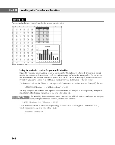
FIGURE 14.6
Frequency distributions created by using the FREQUENCY function
Using formulas to create a frequency distribution
Figure 14.7 shows a worksheet that contains test scores for 50 students in column B (the range is named
Grades). Formulas in columns G and H calculate a frequency distribution for letter grades. The minimum
and maximum values for each letter grade appear in columns D and E. For example, a test score between
80 and 89 (inclusive) earns a B. In addition, a chart displays the distribution of the test scores.

The formula in cell G2 that follows is an array formula that counts the number of scores that qualify for an A:
=COUNTIFS(Grades,”>=”&D2,Grades,”<=”&E2)
You may recognize this formula from a previous section in this chapter (see “Counting cells by using multi-
ple criteria”). This formula was copied to the four cells below G2.
NOTE The preceding formula uses the COUNTIFS function, which is new to Excel 2007. For compat-
NOTE
ibility with previous Excel versions, use this array formula:
{=SUM((Grades>=D2)*(Grades<=E2))}
The formulas in column H calculate the percentage of scores for each letter grade. The formula in H2,
which was copied to the four cells below H2, is
=G2/SUM($G$2:$G$6)

262