Page 399 - Excel 2007 Bible

25_044039 ch19.qxp 11/21/06 11:10 AM Page 356
Part III
Creating Charts and Graphics
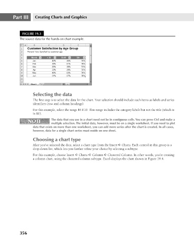
FIGURE 19.3
The source data for the hands-on chart example.
Selecting the data
The first step is to select the data for the chart. Your selection should include such items as labels and series
identifiers (row and column headings).
For this example, select the range B4:E10. This range includes the category labels but not the title (which is
in B1).
NOTE The data that you use in a chart need not be in contiguous cells. You can press Ctrl and make a
NOTE
multiple selection. The initial data, however, must be on a single worksheet. If you need to plot
data that exists on more than one worksheet, you can add more series after the chart is created. In all cases,
however, data for a single chart series must reside on one sheet.
Choosing a chart type
After you’ve selected the data, select a chart type from the Insert ➪ Charts. Each control in this group is a
drop-down list, which lets you further refine your choice by selecting a subtype.
For this example, choose Insert ➪ Charts ➪ Column ➪ Clustered Column. In other words, you’re creating
a column chart, using the clustered column subtype. Excel displays the chart shown in Figure 19.4.

356