Page 64 - Excel 2007 Bible

05_044039 ch01.qxp 11/21/06 10:55 AM Page 21
Introducing Excel
FIGURE 1.18
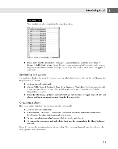
Your worksheet, after converting the range to a table.
4. If you don’t like the default table style, just select another one from the Table Tools ➪ 1
Design ➪ Table Styles group. Notice that you can get a preview of different table styles by mov-
ing your mouse over the ribbon. When you find one you like, click it, and style will be applied to
your table.
Summing the values
The worksheet displays the monthly projected sales, but what about the total sales for the year? Because this
range is a table, it’s simple:
1. Activate any cell in the table
2. Choose Table Tools ➪ Design ➪ Table Style Options ➪ Totals Row. Excel automatically adds
a new row to the bottom of your table, including a formula that calculated the total of the
Projected Sales column.
3. If you’d prefer to see a different summary formula (for example, average), click cell B14 and
choose a different summary formula from the drop-down list.

Creating a chart
How about a chart that shows the projected sales for each month?
1. Activate any cell in the table.
2. Choose Insert ➪ Charts ➪ Column and then select one of the 2-D column chart types.
Excel inserts the chart in the center of your screen.
3. To move the chart to another location, click its border and drag it.
4. To change the appearance and style of the chart, use the commands in the Chart Tools con-
text tab.
Figure 1.19 shows the worksheet after creating the chart. Your chart may look different, depending on the
chart layout or style you selected.

21