Page 63 - Excel 2007 Bible

05_044039 ch01.qxp 11/21/06 10:55 AM Page 20
Part I
Getting Started with Excel
3. The projected sales for subsequent months will use a similar formula. But rather than retype
the formula for each cell in column B, once again take advantage of the AutoFill feature. Make
sure that cell B3 is selected. Click the cell’s fill handle, drag down to cell B13, and release the
mouse button.
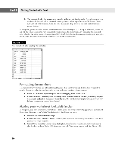
At this point, your worksheet should resemble the one shown in Figure 1.17. Keep in mind that, except for
cell B2, the values in column B are calculated with formulas. To demonstrate, try changing the projected
sales value for the initial month, January (in cell B2). You’ll find that the formulas recalculate and return dif-
ferent values. But these formulas all depend on the initial value in cell B2.
FIGURE 1.17
Your worksheet, after creating the formulas.
Formatting the numbers
The values in the worksheet are difficult to read because they aren’t formatted. In this step, you apply a
number format to make the numbers easier to read and more consistent in appearance:
1. Select the numbers by clicking cell B2 and dragging down to cell B13.
2. Choose Home ➪ Number, click the drop-down Number Format control (it initially displays
General), and select Currency from the list. The numbers now display with a currency sym-
bol and two decimal places. Much better!

Making your worksheet look a bit fancier
At this point, you have a functional worksheet — but it could use some help in the appearance department.
Converting this range to an “official” (and attractive) Excel table is a snap:
1. Move to any cell within the range.
2. Choose Insert ➪ Tables ➪ Table. Excel displays its Create Table dialog box to make sure that it
guessed the range properly.
3. Click OK to close the Create Table dialog box. Excel applies its default table formatting and
also displays its Table Tools ➪ Design contextual tab. Your screen should look like Figure 1.18.

20