Page 297 - Excel for Scientists and Engineers: Numerical Methods

Solving Parabolic Partial Differential Equations:
The Crank-Nicholson or Implicit Method
In the explicit method, we used a central difference formula for the second
derivative and a forward difference formula for the first derivative (equations 12-
24 and 12-25). A variant of equation 12-26 that makes the approximations to
both derivatives central differences is known as the Crank-Nicholson formula
- rKl,,+l + (2 + w4,,+1 - YFf+I,,+I =r%, + (2 - 2r)F,,, + rF,+1,,
(12-27)
or, if i represents distance x and j represents time t,

- rK-l,l+l + (2 + 2m,f+l - r4+1,1+1 = ~~x-I.1 (2 - 2dF,,I + rK+l,*
+
(1 2-27a)
where r = A~/(~(Ax)~). Choosing specific values for r and Ax determines the
increment Ay. For r = 1, equation 12-27a simplifies to equation 12-28.
=
- L,f+l + 4K,l+l - Fx+l,l+l + Fx+~,l ( 12-28)
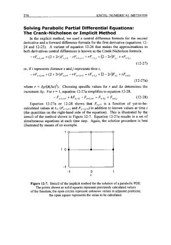
Equation 12-27a or 12-28 shows that Fx,I+l is a function of yet-to-be-
calculated values at t+l (Fx-l,l+l and Fx+l,l+l) in addition to known values at time t
(the quantities on the right-hand side of the equation). This is illustrated by the
stencil of the method shown in Figure 12-7. Equation 12-27a results in a set of
simultaneous equations at each time step. Again, the solution procedure is best
illustrated by means of an example.

-1 0 1
X

Figure 12-7. Stencil of the implicit method for the solution of a parabolic PDE.
The points shown as solid squares represent previously calculated values
of the function; the open circles represent unknown values in adjacent positions;
the open square represents the value to be calculated.