Page 158 - Fair, Geyer, and Okun's Water and wastewater engineering : water supply and wastewater removal

JWCL344_ch04_118-153.qxd 8/2/10 9:18 PM Page 120

120 Chapter 4 Quantities of Water and Wastewater Flows
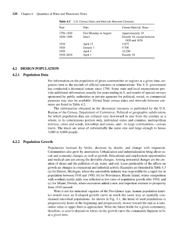
Table 4.2 U.S. Census Dates and Intervals Between Censuses

Year Date Census Interval, Years
1790–1820 First Monday in August Approximately 10
1830–1900 June1 Exactly 10, except between
1820 and 1830
1910 April 15 9.875
1920 January 1 9.708
1930 April 1 10.250
1940–2010 April 1 Exactly 10

4.2 DESIGN POPULATION

4.2.1 Population Data
For information on the population of given communities or regions at a given time, en-
gineers turn to the records of official censuses or enumerations. The U.S. government
has conducted a decennial census since 1790. Some state and local enumerations pro-
vide additional information, usually for years ending in 5, and results of special surveys
sponsored by public authorities or private agencies for political, social, or commercial
purposes may also be available. United State census dates and intervals between cen-
suses are listed in Table 4.2.
The information obtained in the decennial censuses is published by the U.S.
Bureau of the Census, Department of Commerce. Political or geographic subdivisions
for which population data are collated vary downward in size from the country as a
whole, to its coterminous portion only, individual states and counties, metropolitan
districts, cities and wards, townships and towns, and—in large communities—census
tracts. The tracts are areas of substantially the same size and large enough to house
3,000 to 6,000 people.

4.2.2 Population Growth
Populations increase by births, decrease by deaths, and change with migration.
Communities also grow by annexation. Urbanization and industrialization bring about so-
cial and economic changes as well as growth. Educational and employment opportunities
and medical care are among the desirable changes. Among unwanted changes are the cre-
ation of slums and the pollution of air, water, and soil. Least predictable of the effects on
growth are changes in commercial and industrial activity. Examples are furnished in Table 4.3
(a) for Detroit, Michigan, where the automobile industry was responsible for a rapid rise in
population between 1910 and 1950; (b) for Providence, Rhode Island, where competition
with southern textile mills was reflected in low rates of population growth after 1910; and
(c) for Miami, Florida, where recreation added a new and important element to prosperity
from 1910 onward.
Were it not for industrial vagaries of the Providence type, human population kinet-
ics would trace an S-shaped growth curve in much the same way as spatially con-
strained microbial populations. As shown in Fig. 4.1, the trend of seed populations is
progressively faster at the beginning and progressively slower toward the end as a satu-
ration value or upper limit is approached. What the future holds for a given community,
therefore, is seen to depend on where on the growth curve the community happens to be
at a given time.