Page 163 - Fair, Geyer, and Okun's Water and wastewater engineering : water supply and wastewater removal

JWCL344_ch04_118-153.qxd 8/2/10 9:18 PM Page 125

4.2 Design Population 125
services. These are translated into population values by ratios derived for the recent past.
The following ratios are not uncommon:
1. Population: school enrollment 5:1
2. Population: number of water, gas, or electricity services 3:1
3. Population: number of land-line telephone services 4:1

4.2.4 Long-Range Population Forecasts
Long-range forecasts, covering design periods of 10 to 50 years, make use of available and
pertinent records of population growth. Again dependence is placed on mathematical
curve fitting and graphical studies. The logistic growth curve is an example.
The logistic growth equation is derived from the autocatalytic, first-order equation
(Eq. 4.6) by letting
p (L y )>y 0 and q kL
0
or
y L>[l p exp( qt)]
y L>[l exp(ln p qt)]
and equating the first derivative of Eq. 4.1 to zero, or
d(dy>dt)>dt kL 2ky 0
It follows that the maximum rate of growth dy>dt is obtained when

y 1>2L and
t ( ln p)>q ( 2.303 log p)>q

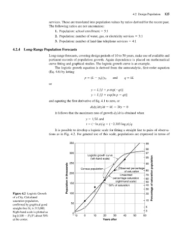
It is possible to develop a logistic scale for fitting a straight line to pairs of observa-
tions as in Fig. 4.2. For general use of this scale, populations are expressed in terms of

350 99
98
300 97
Logistic growth curve
(left-hand scale) Observed percentage 95
250
90
Population in thousands 200 Census population 50% of saturation 80 Percentage of saturation population
of saturation
Linearized
70
percentage saturation
60
(right-hand scale)
50
150
40
Figure 4.2 Logistic Growth 100 30
20
of a City. Calculated
saturation population, 10
50
confirmed by graphical good
5
straight-line fit, is 313,000.
Right-hand scale is plotted as 3
0
log [(100 P)>P] about 50% 10 0 10 20 30 40 50 60
at the center. Years after