Page 317 - Finite Element Modeling and Simulations with ANSYS Workbench

302 Finite Element Modeling and Simulation with ANSYS Workbench

T(x, t)

x

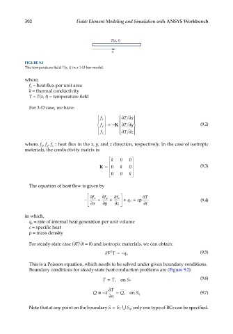
FIGURE 9.1
The temperature field T(x, t) in a 1-D bar model.

where,
f = heat flux per unit area
x
k = thermal conductivity
T = T(x, t) = temperature field

For 3-D case, we have:

∂
 f x  ∂ Tx
   
∂
K
 f y  =−  ∂ Ty  (9.2)
   ∂ Tz 
∂
 f z   
where, f , f , f = heat flux in the x, y, and z direction, respectively. In the case of isotropic
y
z
x
materials, the conductivity matrix is:
k 0  0

K = 0 k 0   (9.3)

0 0  k
 
The equation of heat flow is given by
 ∂T
 ∂f x
∂f y
∂f z
−  + +  + q v = ρ (9.4)
c
 ∂x ∂y ∂z  ∂t
in which,
q = rate of internal heat generation per unit volume
v
c = specific heat
ρ = mass density
For steady-state case (∂T/∂t = 0) and isotropic materials, we can obtain:

k∇ 2 T = − q v (9.5)
This is a Poisson equation, which needs to be solved under given boundary conditions.
Boundary conditions for steady-state heat conduction problems are (Figure 9.2):

T = T,on S T (9.6)
∂ T
Q ≡− k = Q,on S q (9.7)
∂ n

Note that at any point on the boundary S = S T ∪ S q , only one type of BCs can be specified.