Page 321 - Finite Element Modeling and Simulations with ANSYS Workbench

306 Finite Element Modeling and Simulation with ANSYS Workbench

9.3 Modeling of Thermal Problems
Heat transfers in three ways through conduction, convection, and radiation. In FEM,
conduction is modeled by solving the resulting heat balance equations for the nodal
temperatures under specified thermal boundary conditions. Convection is modeled as a
surface load with a user-specified heat transfer coefficient and a given bulk temperature
of the surrounding fluid. Radiation effects, which are nonlinear, are typically modeled
by using the radiation link elements or surface effect elements with the radiation option.
Material properties such as density, thermal conductivity, and specific heat are needed
as input parameters for transient thermal analysis, while steady-state thermal analysis
needs only thermal conductivity as the material input. For thermal stress analysis, mate-
rial input parameters include Young’s modulus, Poisson’s ratio, and thermal expansion
coefficient. In the following, modeling of thermal problems is briefly illustrated with the
aid of two examples.

9.3.1 Thermal Analysis
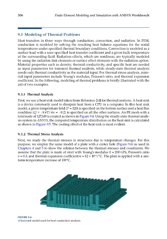
First, we use a heat sink model taken from Reference [14] for thermal analysis. A heat sink
is a device commonly used to dissipate heat from a CPU in a computer. In this heat sink
model, a given temperature field (T = 120) is specified on the bottom surface and a heat flux
∂
condition (Q ≡− k T ∂ n =−0 2) is specified on all the other surfaces. An FE mesh with a
/
.
total node of 127,149 is created as shown in Figure 9.4. Using the steady-state thermal analy-
sis system in ANSYS, the computed temperature distribution on the heat sink is calculated
as shown in Figure 9.5. The cooling effect of the heat sink is most evident.

9.3.2 Thermal Stress Analysis
Next, we study the thermal stresses in structures due to temperature changes. For this
purpose, we employ the same model of a plate with a center hole (Figure 9.6) as used in
Chapters 4 and 5 to show the relation between the thermal stresses and constraints. We
assume that the plate is made of steel with Young’s modulus E = 200 GPa, Poisson’s ratio
ν = 0.3, and thermal expansion coefficient α = 12 × 10 /°C. The plate is applied with a uni-
−6
form temperature increase of 100°C.

FIGURE 9.4
A heat-sink model used for heat conduction analysis.