Page 318 - Finite Element Modeling and Simulations with ANSYS Workbench

Thermal Analysis 303

n
y S q

S T
x

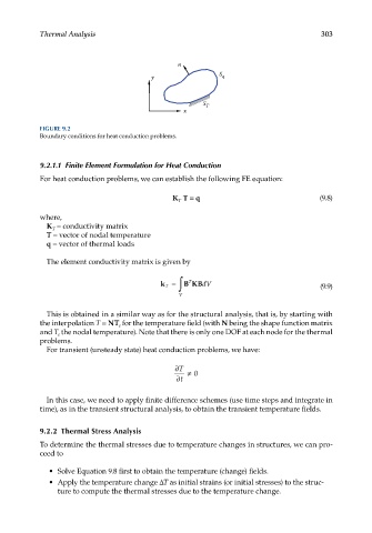
FIGURE 9.2
Boundary conditions for heat conduction problems.

9.2.1.1 Finite Element Formulation for Heat Conduction
For heat conduction problems, we can establish the following FE equation:

K T = q (9.8)
T
where,
K = conductivity matrix
T
T = vector of nodal temperature
q = vector of thermal loads

The element conductivity matrix is given by

k T = ∫ B K BdV (9.9)
T
V

This is obtained in a similar way as for the structural analysis, that is, by starting with
the interpolation T = NT for the temperature field (with N being the shape function matrix
e
and T the nodal temperature). Note that there is only one DOF at each node for the thermal
e
problems.
For transient (unsteady state) heat conduction problems, we have:

∂T ≠ 0
∂t

In this case, we need to apply finite difference schemes (use time steps and integrate in
time), as in the transient structural analysis, to obtain the transient temperature fields.

9.2.2 Thermal Stress Analysis
To determine the thermal stresses due to temperature changes in structures, we can pro-
ceed to

• Solve Equation 9.8 first to obtain the temperature (change) fields.
• Apply the temperature change ΔT as initial strains (or initial stresses) to the struc-
ture to compute the thermal stresses due to the temperature change.