Page 68 - Fluid Mechanics and Thermodynamics of Turbomachinery

Basic Thermodynamics, Fluid Mechanics: Definitions of Efficiency 49
involves a certain degree of arbitrariness and subjectivity on the occurrence of “first
stall”.
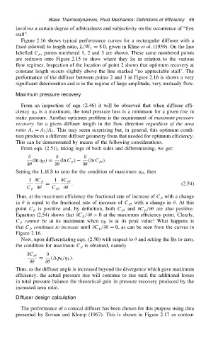
Figure 2.16 shows typical performance curves for a rectangular diffuser with a
fixed sidewall to length ratio, L/W 1 D 8.0, given in Kline et al. (1959). On the line
labelled C p , points numbered 1, 2 and 3 are shown. These same numbered points
are redrawn onto Figure 2.15 to show where they lie in relation to the various
flow regimes. Inspection of the location of point 2 shows that optimum recovery at
constant length occurs slightly above the line marked “no appreciable stall”. The
performance of the diffuser between points 2 and 3 in Figure 2.16 is shows a very
significant deterioration and is in the regime of large amplitude, very unsteady flow.
Maximum pressure recovery

From an inspection of eqn. (2.46) it will be observed that when diffuser effi-
ciency D is a maximum, the total pressure loss is a minimum for a given rise in
static pressure. Another optimum problem is the requirement of maximum pressure
recovery for a given diffuser length in the flow direction regardless of the area
ratio A r D A 2 /A 1 . This may seem surprising but, in general, this optimum condi-
tion produces a different diffuser geometry from that needed for optimum efficiency.
This can be demonstrated by means of the following considerations.
From eqn. (2.51), taking logs of both sides and differentiating, we get:
∂ ∂ ∂
.ln D / D .ln C p / .ln C pi /.
∂ ∂ ∂
Setting the L.H.S to zero for the condition of maximum D , then
1 ∂C p 1 ∂C pi
D . (2.54)
C p ∂ C pi ∂
Thus, at the maximum efficiency the fractional rate of increase of C p with a change
in is equal to the fractional rate of increase of C pi with a change in . At this
point C p is positive and, by definition, both C pi and ∂C p /∂ are also positive.
Equation (2.54) shows that ∂C p /∂ > 0 at the maximum efficiency point. Clearly,
C p cannot be at its maximum when D is at its peak value! What happens is
that C p continues to increase until ∂C p /∂ D 0, as can be seen from the curves in
Figure 2.16.
Now, upon differentiating eqn. (2.50) with respect to and setting the lhs to zero,
the condition for maximum C p is obtained, namely
∂C pi ∂
D .p 0 /q 1 /.
∂ ∂
Thus, as the diffuser angle is increased beyond the divergence which gave maximum
efficiency, the actual pressure rise will continue to rise until the additional losses
in total pressure balance the theoretical gain in pressure recovery produced by the
increased area ratio.
Diffuser design calculation

The performance of a conical diffuser has been chosen for this purpose using data
presented by Sovran and Klomp (1967). This is shown in Figure 2.17 as contour