Page 177 - Fluid-Structure Interactions Slender Structure and Axial Flow (Volume 1)

PIPES CONVEYING FLUID: LINEAR DYNAMICS I 159

A typical Argand diagram is given by Chen (1971a) for ,9 = 0.6, K = 100. In this case
the system loses stability by divergence at u N 4.7, is restabilized at u 2: 7.2, and then
loses stability by single-mode flutter at u N 8.3 - all in the first mode, but at u 2: 17.7
flutter also occurs in the second mode. Thus, this system shares the characteristics of a
cantilevered and a clamped-pinned pipe conveying fluid, with those of the latter being
dominant. For smaller values of K (e.g. K = 10) the system behaves as a cantilever, and
the only possible form of instability is flutter.
Figure 3.62 is the stability diagram in terms of the spring stiffness parameter K. Several
interesting observations may be made: (i) there is a critical value of K, K, = 34.81, below
which only flutter is possible; (ii) for sufficiently high K, there is more than one divergence
region, although the higher ones are of limited physical significance; (iii) for sufficiently
high K (say K > 200), the values of ucf (critical flutter velocities) become significantly less
dependent on ,9 than is the case for low K (say K < 30), as if the system tries to behave
like a conservative one, but still loses stability by flutter: e.g. for ,B = 0.4, 0.5 and 0.6,
and following the second S-shaped curve in the ucf versus ,9 curve (see Figure 3.30) for
,B = 0.7, 0.8 and 0.9; (iv) the three curves shown for B = 0.9 (two of which are dashed)
correspond to loss, recovery and second loss of stability associated with the equivalent
of the third of the S-shaped curves (Figure 3.30).
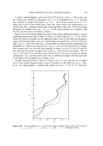
Another interesting result is shown in Figure 3.63. It is seen that the first S-shaped
curve in the stability diagram marks a point of transition for the effect of K on ucf. Thus,
for ,9 < 0.3 approximately, K stabilizes the system vis-&vis K = 0; for ,B > 0.3, however,

16

14

8

6

4
0 0.2 0.4 0.6 0.8 I .0
P

Figure 3.63 The dependence of ucf on #J for the system of Figure 3.61(a) with various values of
K: -, K = 0; -. -. -, K = 10; - - -, K = 50; ---, K = 100 (Chen 1971a).