Page 327 - Fluid-Structure Interactions Slender Structure and Axial Flow (Volume 1)

308 SLENDER STRUCTURES AND AXIAL FLOW

42

41

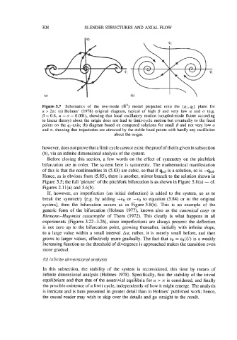
Figure 5.7 Schematics of the two-mode (R4) model projected onto the (ql, q2) plane for
u > 2n: (a) Holmes’ (1978) original diagram, typical of high ,¶ and very low a and u (e.g.
B = 0.8, a = u = 0.001), showing that local oscillatory motion (coupled-mode flutter according
to linear theory) about the origin does not lead to limit-cycle motion but eventually to the fixed
points on the 41-axis; (b) diagram based on computed solutions for small ,¶ and not very low a
and u, showing that trajectories are attracted by the stable fixed points with hardly any oscillation
about the origin.

however, does not prove that a limit cycle cannot exist; the proof of that is given in subsection
(b), via an infinite dimensional analysis of the system.
Before closing this section, a few words on the effect of symmetry on the pitchfork
bifurcation are in order. The system here is symmetric. The mathematical manifestation
of this is that the nonlinearities in (5.83) are cubic, so that if qsol is a solution, so is -qsoI.
Hence, as is obvious from (5.85), there is another, mirror branch to the solution shown in
Figure 5.5; the full ‘picture’ of the pitchfork bifurcation is as shown in Figure 5.8(a) - cf.
Figures 2.11(a) and 5.6(b).
If, however, an imperfection (an initial deflection) is added to the system, so as to
break the symmetry [e.g. by adding +EO or -EO to equation (5.84) or to the original
system], then the bifurcation occurs as in Figure 5.8(b). This is an example of the
generic form of the bifurcation (Holmes 1977), known also as the canonical cusp or
Riemann-Hugoniot catastrophe of Thom (1972). This clearly is what happens in all
experiments (Figures 3.22-3.26), since imperfections are always present: the deflection
is not zero up to the bifurcation point, growing thereafter, initially with infinite slope,
to a large value within a small interval Au; rather, it is merely small before, and then
grows to larger values, effectively more gradually. The fact that EO = EO(U) is a weakly
increasing function as the threshold of divergence is approached makes the transition even
more gradual.
(b) Infinite dimensional analysis

In this subsection, the stability of the system is reconsidered, this time by means of
infinite dimensional analysis (Holmes 1978). Specifically, first the stability of the trivial
equilibrium and then that of the nontrivial equilibria for u > n is considered, and finally
the possible existence of a limit cycle, independently of how it might emerge. The analysis
is intricate and is here presented in greater detail than in Holmes’ published work; hence,
the casual reader may wish to skip over the details and go straight to the result.