Page 506 - Fluid-Structure Interactions Slender Structure and Axial Flow (Volume 1)

476 SLENDER STRUCTURES AND AXIAL FLOW

L?1 being the dimensional first-mode radian frequency. Hence, from the measured 521 and
equation (D.2), the ordinate in Figure D.4 is known, and hence y may be determined;
then, from the definition of y, here mgL3/EZ, so can EZ. Similarly, from the measured 81
and Figure D.3, p + &e(wl) may be found. Thus, p may be determined if the damping
is supposed to be purely hysteretic (a = 0); and so can a, if p = 0 is taken. If both
are required for a more realistic representation of the damping, then two experiments are
necessary with different pipes, e.g. pipes of different length.
The robustness of a particular damping model may be assessed by determining p andor
a for second- and third-mode vibration also, and then utilizing another figure for these
higher modes, similar to Figure D.4 and given in Pdidoussis & Des Trois Maisons (1971).
In some cases, rather than commit oneself to a particular damping model, 81, 82, 83
and so on are determined separately and used directly when comparing with theory - see
Section D.4.
Finally, to determine the Poisson ratio, u, a sufficiently large cube of silicone rubber
is cast, and is then weighed down with progressively heavier blocks, while its vertical
compression and lateral expansion are measured with dial gauges and fibre-optic sensors.

D.4 MEASUREMENT OF FREQUENCIES AND DAMPING

Many different ways for measuring the damping are possible, but the methods described
here are both simple and efficient. The following pieces of equipment are required: (i) a
sensor, (ii) a signal recording device; also, optional but very useful are (iii) a small shaker,
(iv) a band-pass filter, and (v) a digital signal analyser.
Exciting the pipe by flexing it and then releasing it generally works well for the first
mode only. Trying to excite the second and third modes in this way is difficult if not

0 8
Time (s)
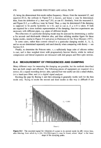
Figure D.5 The recorded signal for vibration of a pipe in its second mode (in dB) versus time,
after filtering, from which 82 = [(ln 10)/20](slope)/f2 may be found, where ‘slope’ is the linear
slope of the decaying peaks.