Page 410 - T. Anderson-Fracture Mechanics - Fundamentals and Applns.-CRC (2005)

1656_C009.fm Page 390 Monday, May 23, 2005 3:58 PM

390 Fracture Mechanics: Fundamentals and Applications

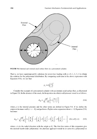
FIGURE 9.6 Internal and external axial surface flaws in a pressurized cylinder.

That is, we have superimposed K solutions for power-law loading with n = 0, 1, 2, 3, 4 to obtain
I
the solution for the polynomial distribution. By comparing each term in the above expression with
Equation (9.6), we see that

p = σ n  a  n
t  
n
Consider the example of a pressurized cylinder with an internal axial surface flaw, as illustrated
in Figure 9.6. In the absence of the crack, the hoop stress in a thick wall pressure vessel is as follows:

pR 2   R  2 
σ θθ = R o 2 − R i i 2  1 +  r o    (9.8)


where p is the internal pressure and the other terms are defined in Figure 9.6. If we define the
origin at the inner wall (x = r – R) and perform a Taylor series expansion about x = 0, Equation (9.8)
i
becomes

pR 2   R  2  x   x  2  x  3  x  4 
σ θθ = R o 2 − R o i 2 1 +   R o i   − 2   R i   + 3   R i   − 4   R i   + 5   R i   +    0 ( ≤ i ≤ xR / 1) (9.9)



where x is in the radial direction with the origin at R . The first five terms of this expansion give
i
the desired fourth-order polynomial. An alternate approach would be to curve-fit a polynomial to