Page 411 - T. Anderson-Fracture Mechanics - Fundamentals and Applns.-CRC (2005)

1656_C009.fm Page 391 Monday, May 23, 2005 3:58 PM

Application to Structures 391

the stress field. This latter method is necessary when the stress distribution does not have a closed-
form solution, such as when nodal stresses from a finite element analysis are used.
When computing K for the internal surface flaw, we must also take account of the pressure
I
loading on the crack faces. Superimposing p on Equation (9.9), and applying Equation (9.7) to
each term in the series leads to the following expression for K [7,12]:
I
pR 2   a   a  2  a  3  a  4  π a
K = R 2 o o R − i 2 2 G − 2   R   G + 3   R   G − 4   R   G + 5   R   G    Q (9.10)
o
I
1
i 
2
4
3

i
i
i
Applying a similar approach to an external surface flaw leads to
pR 2   a   a  2  a  3  a  4  π a
K = R o 2 i R − i 2 2 G + 2   R   G + 3   R   G + 4   R   G + 5   R   G    Q (9.11)
o
I
1
3
o 
2
4

o
o
o
The origin in this case was defined at the outer surface of the cylinder, and a series expansion was
performed as before. Thus K for a surface flaw in a pressurized cylinder can be obtained by
I
substituting the appropriate influence coefficients into Equation (9.10) or Equation (9.11).
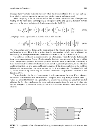
The influence coefficient approach is useful for estimating K values for cracks that emanate
I
from stress concentrations. Figure 9.7 schematically illustrates a surface crack at the toe of a fillet
weld. This geometry produces local stress gradients that affect the K for the crack. Performing a
I
finite element analysis of this structural detail with a crack is generally preferable, but the influence
coefficient method can give a reasonable approximation. If the stress distribution at the weld toe
is known for the uncracked case, these stresses can be fit to a polynomial (Equation (9.6)), and
K can be estimated by substituting the influence coefficients and polynomial coefficients into
I
Equation (9.7).
The methodology in the previous example is only approximate, however. If the influence
coefficients were obtained from an analysis of a flat plate, there may be slight errors if these G n
values are applied to the fillet weld geometry. The actual weld geometry has a relatively modest
effect on the G values. As long as the stress gradient emanating from the weld toe is taken into
n
account, computed K values will usually be within 10% of values obtained from a more rigorous
I
analysis.

FIGURE 9.7 Application of the influence coefficient approach to a complex structural detail such as a fillet
weld.