Page 30 - Fundamentals of Computational Geoscience Numerical Methods and Algorithms

16 2 Simulating Steady-State Natural Convective Problems

S(Ra, α)
α = α 1

α = α 2

α = α
n
α is too small

0
Ra critical Ra
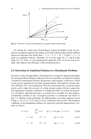
Fig. 2.1 The basic concept of the progressive asymptotic approach procedure

For solving the steady-state Horton-Rogers-Lapwood problem using the pro-
gressive asymptotic approach procedure associated with the finite element method,
numerical experience has shown that 1 ≤ α ≤ 5 ,5 ≤ R ≤ 10 and 1 ≤ n ≤ 2
◦
◦
leads to acceptable solutions. Therefore, for α in the range of 1–5 and R in the
◦
range of 5–10, S(Ra,α) can asymptotically approach S(Ra, 0) in one step or two
steps. This indicates the efficiency of the present procedure.

2.4 Derivation of Analytical Solution to a Benchmark Problem

In order to verify the applicability of the progressive asymptotic approach procedure
for solving the Horton-Rogers-Lapwood convection problem, an analytical solution
is needed for a benchmark problem, the geometry and boundary conditions of which
can be exactly modelled by the finite element method. Although the existing solu-
tions (Phillips 1991, Nield and Bejan 1992) for a horizontal layer in porous media
can be used to check the accuracy of a finite element solution within a square box
with appropriate boundary conditions, it is highly desirable to examine the progres-
sive asymptotic approach procedure as extensively as possible. For this purpose,
a benchmark problem of any rectangular geometry is constructed and shown in
Fig. 2.2. Without losing generality, the dimensionless governing equations given
in Eqs. (2.10), (2.11), (2.12) and (2.13) are considered in this section. The boundary
conditions of the benchmark problem are expressed using the dimensionless vari-
ables as follows:
∂T ∗
∗
∗
∗
∗
u = 0, = 0 (at x = 0 and x = L ), (2.46)
∂x ∗
∗
∗
∗
v = 0, T = 1 (at y = 0), (2.47)
∗
∗
∗
v = 0, T = 0 (at y = 1), (2.48)