Page 31 - Fundamentals of Computational Geoscience Numerical Methods and Algorithms

2.4 Derivation of Analytical Solution to a Benchmark Problem 17

1
y *
x *
0
L *

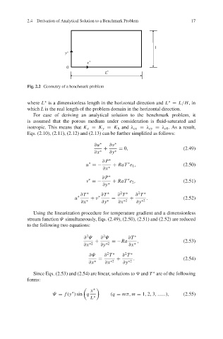
Fig. 2.2 Geometry of a benchmark problem

∗
where L is a dimensionless length in the horizontal direction and L = L/H,in
∗
which L is the real length of the problem domain in the horizontal direction.
For ease of deriving an analytical solution to the benchmark problem, it
is assumed that the porous medium under consideration is fluid-saturated and
isotropic. This means that K x = K y = K h and λ ex = λ ey = λ e0 . As a result,
Eqs. (2.10), (2.11), (2.12) and (2.13) can be further simplified as follows:

∂u ∗ ∂ν ∗
+ = 0, (2.49)
∂x ∗ ∂y ∗
∂ P ∗
∗ ∗
u =− + RaT e 1 , (2.50)
∂x ∗
∂ P ∗
∗ ∗
v =− + RaT e 2 , (2.51)
∂y ∗
2
2
∂T ∗ ∂T ∗ ∂ T ∗ ∂ T ∗
u ∗ + ν ∗ = + . (2.52)
∂x ∗ ∂y ∗ ∂x ∗2 ∂y ∗2
Using the linearization procedure for temperature gradient and a dimensionless
stream function Ψ simultaneously, Eqs. (2.49), (2.50), (2.51) and (2.52) are reduced
to the following two equations:

2
2
∂ Ψ ∂ Ψ ∂T ∗
+ =−Ra , (2.53)
∂x ∗2 ∂y ∗2 ∂x ∗
2
2
∂Ψ ∂ T ∗ ∂ T ∗
= + . (2.54)
∂x ∗ ∂x ∗2 ∂y ∗2
∗
Since Eqs. (2.53) and (2.54) are linear, solutions to Ψ and T are of the following
forms:
x
∗
∗
Ψ = f (y )sin q (q = mπ, m = 1, 2, 3, ......), (2.55)
L ∗