Page 153 - Fundamentals of Gas Shale Reservoirs

WELL LOG ANALYSIS OF GAS SHALE RESERVOIRS 133
(a) (b)
1 1

0.8 0.8

BI mineralogy 0.6 R = 0.80 BI mineralogy 0.6 R = 0.78

0.4
2
2
0.4
0.2 0.2
0 0
0 0.2 0.4 0.6 0.8 1 0 0.2 0.4 0.6 0.8 1
BI
BI sonic sonic
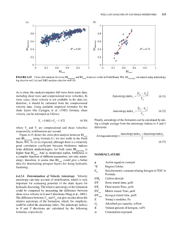
FIGURE 6.15 Cross‐plot analysis between BI mineralogy and BI sonic from two wells in Perth Basin, WA. BI mineralogy calculated using mineralogy
log data for well (a) and XRD analysis data for well (b).

As is clear, this analysis requires full wave‐form sonic data, V – V
including shear wave and compressional wave velocities. In Anisotropyindex x sx sy (6.31)
some cases, shear velocity is not available in the data set; V sx
therefore, it should be estimated from the compressional
velocity data. Using available empirical formulas for the V – V
shale layers like Castagna et al. (1985) formula, shear Anisotropyindex sx sy (6.32)
velocity can be estimated as follows: y V sy

V 0 862 V 1 172 (6.30) Finally, anisotropy of the formation can be calculated by tak­
.
.
s p
ing a simple average from the anisotropy indices in X and Y
where V and V are compressional and shear velocities directions:
p
s
respectively, in kilometers per second.
Figure 6.15 shows the cross‐plot analysis between BI sonic Averageanisotropy Anisotropyindex x Anisotropyindex y
and BI mineralogy using formula 6.1 for two wells in the Perth 2
Basin, WA. As (it is) expected, although there is a relatively (6.33)
good correlation coefficient between brittleness indexes
from different methodologies, for both cases BI mineralogy is
higher than BI sonic . And as mentioned earlier, brittleness is NOMENCLATURE
a complex function of different parameters, not only miner­
alogy; therefore, it seems that BI sonic could give a better
idea for determining prospect layers for doing hydraulic a Archie equation constant
fracturing. °C Degree Celsius
C Stoichiometric constant relating kerogen to TOC in
k
Formula
6.4.2.6 Determination of Velocity Anisotropy Velocity
anisotropy can take account of stratification, which is very CO Carbon dioxide
2
important for evaluating potential of the shale layers for DT Sonic transit time, μs/ft
hydraulic fracturing. The relative anisotropy of the formation DT Fluid transit Time, μs/ft
f
could be computed by measuring the difference between DT Matrix transit Time, μs/ft
shear wave velocity in X and Y directions (Tang et al., 2001). DT ma Kerogen transit time, μs/ft
The difference between V and V can give an idea about the E TOC Young’s modulus, Pa
sx
sy
relative anisotropy of the formation, which, for simplicity,
could be called the anisotropy index. The anisotropy indices G Adsorbed gas capacity, scf/ton
s
in X and Y directions are calculated by the following K Volume percent of kerogen, vol%
formulas, respectively: m Cementation exponent