Page 168 - Fundamentals of Gas Shale Reservoirs

148 PORE PRESSuRE PREdIcTIOn FOR ShAlE FORmATIOnS uSInG WEll lOG dATA

It should be noted that the aforementioned correlations were n
derived based on an empirical basis for Gulf of mexico data tak- ob b gdz (7.11)
ing into consideration the overpressure‐generating mechanism i 1
in disequilibrium compaction. For this reason, it is also impor- 4
tant to note that this method does not imply the particular over- v b (7.12)
.
pressure‐generating mechanisms, whether loading or unloading. 023
Eaton (1975) also did not mention in his study how to determine
the ncT; however, experience indicates that normal compac- where σ is the overburden stress gradient given in
ob
tion trend curves can be established for sediments with normal psi/ft, ρ in the bulk density given in g/cm , g is the
3
b
pressure overlying the overpressured sections. gravitational acceleration, and z is the vertical depth
to the formation given in meters, v is the velocity
7.3.2.1 Hints for Using Eaton’s Method which is the inverse of sonic transit time and is given
• Establish relationships of depth versus the porosity‐ in ft/s, and the constants 0.23 and 4 are derived
dependent parameters, for example, logarithm of shale empirically.
sonic transit time or shale resistivity for normally pres- 2. Establish the relationship between sonic transit time
sured formations. versus depth for hydrostatic‐pressure formations
• Establish the normal compaction trend in normally (Fig. 7.12).
pressured clean shale. 3. Establish the normal compaction trend for sonic
• On sonic transit time versus depth plot, the observed log and observe any departure of transit time
relationship will be generally a linear relationship. from the established normal compaction trend
• On resistivity versus depth plot, the observed relation- (Fig. 7.12).
ship will be a nonlinear relationship. Estimate the pore pressure using the relevant Eaton’s
• The departure of data from normal compaction trends correlation (Eq. 7.7 and Fig. 7.13).
is used as a measure of pore pressure within the shale. This real example was taken from Perth Basin in Western
Australia. After testing different values for the x exponent in
Example: Eaton’s correlation (Eq. 7.7), the study concluded that the
using Eaton’s method (sonic), estimate pore pressure best match between the estimated pore pressures and other
gradient at depth of 3576 m TVd for Well #2. relevant data could be found when using a value of 1.5 for
Steps as shown in Figure 7.12: the x exponent.

1. Generate overburden gradient from the density log.
The overburden stress is computed from the density 15
.
log which measures the bulk density every 0.152 m. g p g ob g ob g n t n
Thus, the calculation of the overburden stress is made t o
at every depth step. The overburden stress is computed 65 74 15 .
.
.
.
.
by using the Equation 7.11, and examples of these g p 0 997 0 997 0 433 7 79 66
.
calculations are shown in Table 7.1.
/
.
note: If the density log is not available, generate g p 0 574psift
the density log from sonic transit time by using p at 3576mTVD
p
Gardner’s method (Gardner et al., 1974) (Eq. 7.12) or 0 574 3576 32881 6733psi
.
.
the other available methods. p p
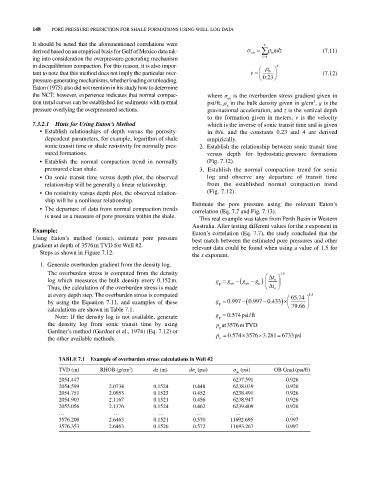
TAbLE 7.1 Example of overburden stress calculations in Well #2
TVd (m) RhOB (g/cm ) dz (m) dσ (psi) σ (psi) OB Grad (psi/ft)
3
v ob
2054.447 6237.591 0.926
2054.599 2.0734 0.1524 0.448 6238.039 0.926
2054.751 2.0953 0.1523 0.452 6238.491 0.926
2054.903 2.1167 0.1521 0.456 6238.947 0.926
2055.056 2.1376 0.1524 0.462 6239.409 0.926
… … … … … …
3576.200 2.6463 0.1521 0.570 11692.695 0.997
3576.353 2.6463 0.1526 0.572 11693.267 0.997