Page 92 - Fundamentals of Gas Shale Reservoirs

72 SEQUENCE STRATIGRAPHY OF UNCONVENTIONAL RESOURCE SHALES

(a) sequence stratigraphic model (Haq et al., 1984). In an earlier
Geologic time
High paper, Slatt and Rodriguez (2012) suggested a stratigraphic
Sea level Valley carved Valley lled commonality among the resource shales and provided a
Falling Rising general sequence stratigraphic model that is applicable to
Falling stage sea level (regression)
Low
limb limb
One sea level cycle
SB shales at a variety of chronostratigraphic scales. In this
IV SL
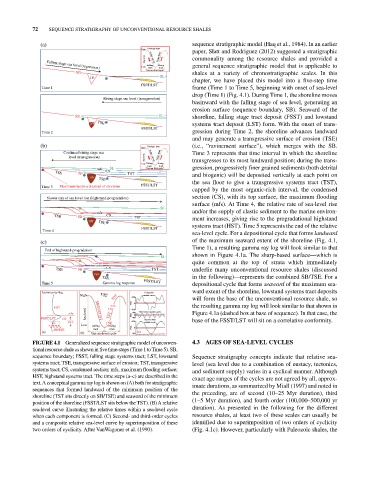
chapter, we have placed this model into a five‐step time
FSST/LST
Time 1 frame (Time 1 to Time 5, beginning with onset of sea‐level
drop (Time 1) (Fig. 4.1). During Time 1, the shoreline moves
Rising stage sea level (transgression)
basinward with the falling stage of sea level, generating an
erosion surface (sequence boundary, SB). Seaward of the
SB SL shoreline, falling stage tract deposit (FSST) and lowstand
IVF TSE systems tract deposit (LST) form. With the onset of trans­
FSST/LST
Time 2 gression during Time 2, the shoreline advances landward
and may generate a transgressive surface of erosion (TSE)
(b) (i.e., “ravinement surface”), which merges with the SB.
High Geologic time
Continued rising stage sea Time 3 represents that time interval in which the shoreline
level (transgression) Sea level Valley carved Valley lled transgresses to its most landward position; during the trans­
Low Falling Rising
limb limb gression, progressively finer grained sediments (both detrital
mfs SL One sea level cycle
TSE SB CS TST and biogenic) will be deposited vertically at each point on
IVF
TSE
the sea floor to give a transgressive systems tract (TST),
Time 3 Maximum landward extent of shoreline FSST/LST
capped by the most organic‐rich interval, the condensed
Slower rate of sea level rise (highstand-progradation) section (CS), with its top surface, the maximum flooding
surface (mfs). At Time 4, the relative rate of sea‐level rise
SL
mfs and/or the supply of clastic sediment to the marine environ­
TSE SB CS TST ment increases, giving rise to the progradational highstand
IVF TSE
systems tract (HST). Time 5 represents the end of the relative
FSST/LST
Time 4
sea‐level cycle. For a depositional cycle that forms landward
(c) of the maximum seaward extent of the shoreline (Fig. 4.1,
Time 1), a resulting gamma ray log will look similar to that
End of highstand-progradation
SL shown in Figure 4.1a. The sharp‐based surface—which is
quite common at the top of strata which immediately
mfs
TSE SB CS TST underlie many unconventional resource shales (discussed
IVF in the following)—represents the combined SB/TSE. For a
TSE
Time 5 Gamma log response FSST/LST depositional cycle that forms seaward of the maximum sea­
Gamma-ray log Composite ward extent of the shoreline, lowstand systems tract deposits
High Time eustatic curve
HST +100 will form the base of the unconventional resource shale, so
Feet 0
mfs the resulting gamma ray log will look similar to that shown in
HST CS –100
mfs Sea level SB/FSST/ST TST +40 Third order eustatic cycle Figure 4.1a (dashed box at base of sequence). In that case, the
FSST/LST CS Feet –40 0 Second order base of the FSST/LST will sit on a correlative conformity.
TST TSE +100 eustatic cycle
Low Falling Rising
SB/TSE limb limb Feet 0
(a) (b) One sea level cycle –100 (c)
FIGurE 4.1 Generalized sequence stratigraphic model of unconven­ 4.3 aGES OF SEa‐LEVEL CyCLES
tional resource shale as shown in five time‐steps (Time 1 to Time 5). SB,
sequence boundary; FSST, falling stage systems tract; LST, lowstand Sequence stratigraphy concepts indicate that relative sea‐
systems tract; TSE, transgressive surface of erosion; TST, transgressive level (sea level due to a combination of eustacy, tectonics,
systems tract; CS, condensed section; mfs, maximum flooding surface; and sediment supply) varies in a cyclical manner. Although
HST, highstand systems tract. The time steps (a–c) are described in the exact age ranges of the cycles are not agreed by all, approx­
text. A conceptual gamma ray log is shown on (A) both for stratigraphic imate durations, as summarized by Miall (1997) and noted in
sequences that formed landward of the minimum position of the
shoreline (TST sits directly on SB/TSE) and seaward of the minimum the preceding, are of second (10–25 Myr duration), third
position of the shoreline (FSST/LST sits below the TST). (B) A relative (1–5 Myr duration), and fourth order (100,000–500,000 yr
sea‐level curve illustrating the relative times within a sea‐level cycle duration). As presented in the following for the different
when each component is formed. (C) Second‐ and third‐order cycles resource shales, at least two of these scales can usually be
and a composite relative sea‐level curve by superimposition of these identified due to superimposition of two orders of cyclicity
two orders of cyclicity. After VanWagoner et al. (1990). (Fig. 4.1c). However, particularly with Paleozoic shales, the