Page 379 - Fundamentals of Magnetic Thermonuclear Reactor Design

Mechanics of Magnetic Fusion Reactors Chapter | 12 357

winding is treated as a homogeneous anisotropic object whose properties have
been determined at the first stage. A numerical analysis is performed using
standard computer simulation tools, such as ANSYS. Applying ponderomotive
forces to the nodes of the model mesh is a separate task, as these forces can
be determined using special software and meshes different from those used
in strength calculations. As a result, we obtain the stress–strain state of load-
bearing structures and average strain field, as well as deformations of the com-
posite structures.
At the third stage, we get back to the local finite-element model of the cell.
Actual stresses and deformations in coil materials, needed to estimate the struc-
ture’s strength and life-time, are determined by superimposing benchmark
problem solutions, corrected for obtained effective deformations. To illustrate
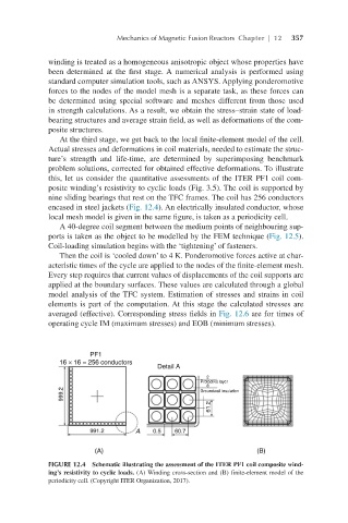
this, let us consider the quantitative assessments of the ITER PF1 coil com-
posite winding’s resistivity to cyclic loads (Fig. 3.5). The coil is supported by
nine sliding bearings that rest on the TFC frames. The coil has 256 conductors
encased in steel jackets (Fig. 12.4). An electrically insulated conductor, whose
local mesh model is given in the same figure, is taken as a periodicity cell.
A 40-degree coil segment between the medium points of neighbouring sup-
ports is taken as the object to be modelled by the FEM technique (Fig. 12.5).
Coil-loading simulation begins with the ‘tightening’ of fasteners.
Then the coil is ‘cooled down’ to 4 K. Ponderomotive forces active at char-
acteristic times of the cycle are applied to the nodes of the finite-element mesh.
Every step requires that current values of displacements of the coil supports are
applied at the boundary surfaces. These values are calculated through a global
model analysis of the TFC system. Estimation of stresses and strains in coil
elements is part of the computation. At this stage the calculated stresses are
averaged (effective). Corresponding stress fields in Fig. 12.6 are for times of
operating cycle IM (maximum stresses) and EOB (minimum stresses).

FIGURE 12.4 Schematic illustrating the assessment of the ITER PF1 coil composite wind-
ing’s resistivity to cyclic loads. (A) Winding cross-section and (B) finite-element model of the
periodicity cell. (Copyright ITER Organization, 2017).