Page 303 - Fundamentals of Ocean Renewable Energy Generating Electricity From The Sea

288 Fundamentals of Ocean Renewable Energy

based on Eq. (10.5). In particular, opposing currents can increase wave height
and wave steepness. This can lead to wave breaking. Referring to Eq. (10.4), the
wave group velocity will be reduced by opposing currents. If tidal currents are
strong enough, the group velocity approaches zero, which means that waves can
be completely blocked by currents.
The discussion above was based on a simplified method to help understand
the concepts. In real applications, several ocean models offer coupled wave and
tide modelling capability. These models can be used to simulate the interactions
of waves and tides. For instance, SWAN has been coupled with both ADCIRC
and ROMS models (introduced in Chapter 8). SWAN can include the effect of
tidal currents on wave power by importing the tidal current and elevation fields
from a tidal model (e.g. ADCIRC or ROMS).

Effect of Waves on the Tidal Energy Resource
Energetic waves can alter tidal currents and tidal elevations. For instance, waves
add additional momentum/force to the tidal flow (i.e. wave radiation stresses).
Further, the interaction of wave orbital velocities and the bottom boundary
layer (of currents) leads to an increase in the roughness felt by currents.
The enhancement of bed roughness due to wave-current interaction has been
estimated as [28]

U w 2
k a = k s exp Γ < 10, Γ = 0.80 + φ − 0.3φ (10.6)
u
in which k a is the apparent roughness, k s is the physical roughness, u is the
current velocity, U w is the near-bed wave-induced orbital velocity, and φ is
the angle between wave and current directions (in radians). As this equation
demonstrates, the apparent bed roughness can be much higher (up to 10 times)
than the physical bed roughness. In tidal models, friction coefficients such as
drag or Manning’s are used to represent the bottom friction rather than the bed
roughness. For the drag coefficient, it can be shown that [26,29]
3.2
C * λ τ w
γ = D = 1 + 1.2 < 2.2, λ = (10.7)
C D 1 + λ τ c
*
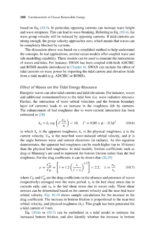
where C D and C are the drag coefficients in the absence and presence of waves
D
(respectively) averaged over the wave period. τ c is the bed shear stress due to
currents only, and τ w is the bed shear stress due to waves only. These shear
stresses can be determined based on the current velocity and the near-bed wave
orbital velocity. Fig. 10.10 shows sample calculations for the increase in the
drag coefficient. The increase in bottom friction is proportional to the near-bed
orbital velocity, and physical roughness (k s ). This graph has been generated for
a tidal current of 1 m/s.
Eq. (10.6) or (10.7) can be embedded in a tidal model to estimate the
increased bottom friction, and also identify whether the increase in bottom