Page 317 - Fundamentals of Probability and Statistics for Engineers

300 Fundamentals of Probability and Statistics for Engineers

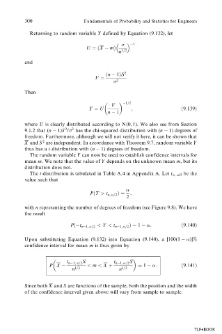
Returning to random variable Y defined by Equation (9.132), let

1
U ˆ X m†
n 1=2
and

n 1†S 2
V ˆ
2
Then

1=2

V
Y ˆ U ; 9:139†
n 1
where U is clearly distributed according to N(0, 1). We also see from Section
2
9.1.2 that (n 1)S / 2 has the chi-squared distribution with (n 1) degrees of
freedom. Furthermore, although we will not verify it here, it can be shown that
X and S are independent. In accordance with Theorem 9.7, random variable Y
2
thus has a t-distribution with (n 1) degrees of freedom.
The random variable Y can now be used to establish confidence intervals for
mean m. We note that the value of Y depends on the unknown mean m, but its
distribution does not.
The t-distribution is tabulated in Table A.4 in Appendix A. Let t n, /2 be the

value such that

P T > t n; =2 †ˆ ;
2
with n representing the number of degrees of freedom (see Figure 9.8). We have
the result

P t n 1; =2 < Y < t n 1; =2 †ˆ 1 : 9:140†

Upon substituting Equation (9.132) into Equation 9.140), a [100 1 )]%
confidence interval for mean m is thus given by

t n 1; =2 S t n 1; =2 S

P X < m < X ‡ ˆ 1 : 9:141†
n 1=2 n 1=2

Since both X and S are functions of the sample, both the position and the width
of the confidence interval given above will vary from sample to sample.

TLFeBOOK