Page 335 - Fundamentals of Probability and Statistics for Engineers

318 Fundamentals of Probability and Statistics for Engineers

Let us note that D is a statistic since it is a function of N i , which are, in turn,
functions of sample X 1 ,..., X n . The distribution of statistic D is given in
Theorem 10.1, attributable to Pearson (1900).
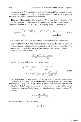
Theorem 10.1: assuming that hypothesis H is true, the distribution of D

defined by Equation (10.4) approaches a chi-squared distribution with (k 1)
degrees of freedom as n!1 . Its pdf is given by [see Equation (7.67)]
8
h i 1
2 d e ; for d 0;
< k 1†=2 k 1 k 3†=2 d=2
f d†ˆ 2 10:5†
D
0; elsewhere.
:
Note that this distribution is independent of the hypothesized distribution.
 e
Proof of Theorem 10.1: The complete proof, which can be found in Cram er
(1946) and in other advanced texts in statistics, will not be attempted here. To
demonstrate its plausibility, we only sketch the proof for the k ˆ 2 case.
For k ˆ 2, random variable D is

N 1 np 1 † 2 N 2 np 2 † 2
D ˆ ‡ :
np 1 np 2

Since N 1 ‡ N 2 ˆ n, and p 1 ‡ p 2 ˆ 1, we can write

N 1 np 1 † 2 ‰n N 1 n 1 p 1 †Š 2
D ˆ ‡
np 1 np 2
10:6†
2
1 1 N 1 np 1 †
2
ˆ N 1 np 1 † ‡ ˆ :
np 1 np 2 np 1 1 p 1 †
Now, recalling that N 1 is the number of, say, successes in n trials, with p 1 being
the probability of success, it is a binomial random variable with EfN 1 gˆ np 1
and varfN 1 gˆ np 1 -1 p 1 ) if hypothesis H is true. As n increases, we have seen
in Chapter 7 that N 1 approaches a normal distribution by virtue of the central
limit theorem (Section 7.2.1). Hence, the distribution of random variable U,
defined by
N 1 np 1
U ˆ ;
‰np 1 1 p 1 †Š 1=2

approaches N(0, 1) as n !1 . Since

2
D ˆ U ;

TLFeBOOK